

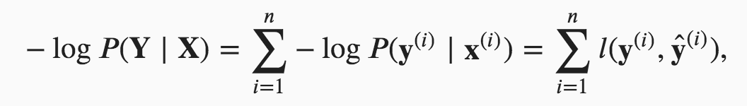
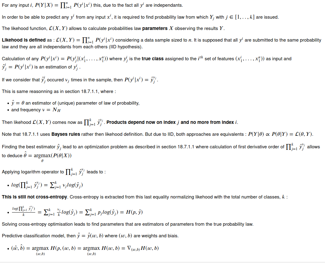
The first part is the definition of the joint likelihood function:
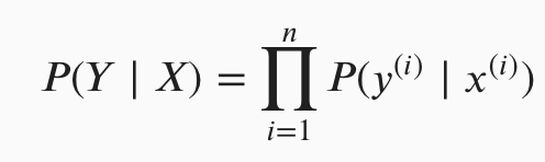
How likely it is that we observe the classifications that we do, conditional on the the input data we have and the parameters we choose (the full version of this should include the parameters after x in some form I think). We’re trying to maximise this: to choose the parameters that make the combination of input data & actual labels that we observed as likely as possible.
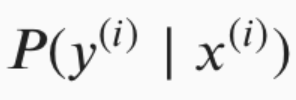
The second part is just a mathematical manipulation of the first part:
<image of the second part that I can’t insert because I’m new  )
)
So we can note that maximising the first is the same as minimising the second (since we took the negative of it), and therefore we can treat the second as a ‘loss function’ (thing we want to minimise).
1 reply
Thanks. I already have known what -log does. But I still wonder the math meaning and, more importantly , realistic meaning of the definition of the joint likelihood function.

Why would we need to multiply all P(y|x)
 ?
?
Do their parameters independent surely?
If we multiply some numbers which stands for different meanings, the meaning of the result is hard to say.
And I think probability is often illusive if we only use pure math without any other descripition of a natural language.
1 reply
Hi @StevenJokes,
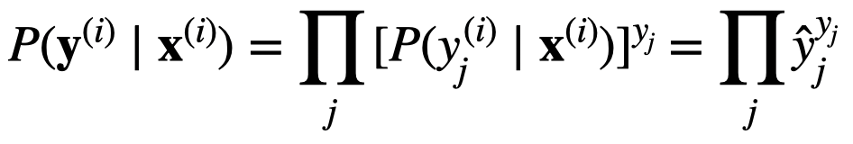
$P(Y | X) = P(y_1, y_2, … | x_1,x_2,…) = \prod{P(y_i | x_i)}$ since the samples are independent.
Are we sure about the independence? How can we? Or we just naively think that all samples are independent?
I think that independence and the establish of $P(Y | X) = P(y_1, y_2, … | x_1,x_2,…) = \prod{P(y_i | x_i)}$ 's equal sign are mutual causation.In other words, just logical rename.
Thanks. But I think I’m still confused. Are we sure about the independence? How can we? Or we just naively think that all samples are independent?
I think that independence and the establish of $P(Y | X) = P(y_1, y_2, … | x_1,x_2,…) = \prod{P(y_i | x_i)}$ 's equal sign are mutual causation. In other words, just logical rename. We should know what P*P refers in the real world. 
And I think probability just refers to how much fraction of some real whole thing, but we use it abusely to try to predict, such as whether head or tail a coin will face up nextly.
And it is understandable to use it to process natural language due to consistency required in Logic.
But we still need more information to predict a dynamic process. And we just want to be a peacemaker when we say that P = 1/2, then we will be confident to not be wrong too much.
And we can’t predict any if we can’t describe what will happen and what situation we are in now.
And different ways to describe a thing usually confuses each other, then another story will happen.
The attempts to simplify our world by concluding everything maybe just deduce a contrary result that the world will be more complex due to typo, syntax error, lie, misunderstanding, distrust and so on. 
Just my random thoughts. 
I think we do assume that the samples are conditionally independent yes - after conditioning on the input data x_i, the y_i values are independent of each other. I think this comes from assuming that the Gaussian noise in the model is well-behaved (iid).
The book has more to say on this in section 4.4.1.1:
In the standard supervised learning setting, which we have addressed up until now and will stick with throughout most of this book, we assume that both the training data and the test data are drawn independently from identical distributions (commonly called the i.i.d. assumption). This means that the process that samples our data has no memory.
1 reply
No memory is too abstract. What does it mean?
I need more examples of identical distrbutions.
What can we call that they are identical distributions?
For example, students in a class are identical distributions?
But they usually have similiar ages and live near the school.
I read an example of it:
Just like if I flip the dice and I flip it every time, that’s independent. But if I want the sum of the two flips to be greater than 8, and the rest doesn’t count, then the first flip and the second flip are not independent, because the second flip is dependent on the first flip
What I want globally will change the dependence of data itself. Am I right?
If so, I can say it is dependent or not, just by my thought.
And I think the probablity is just an ideal thought by some mathematicians who has crazy thought to predict everything just by math.
1 reply
So, we only wait for the result of the second to happen?
Probability, in the begining, more depends on what we think how many categories result are.
And, because we have freedom to say, inconsistency is so common, such as famous “Bayesian method”.
Bayesian method actually looks like a good way that we try to put right after finding something wrong.
But it is hard to say that, what we tried to fix in past will be still effective in the future. ![]()
Again, my random thought!
If we can fully use the past experience to guide our action in future, then how similar of past and future is the next question that we should take attention to.
In my understanding,
over-fitting problems focus more on difference of past and future, while
under-fitting on similarity.

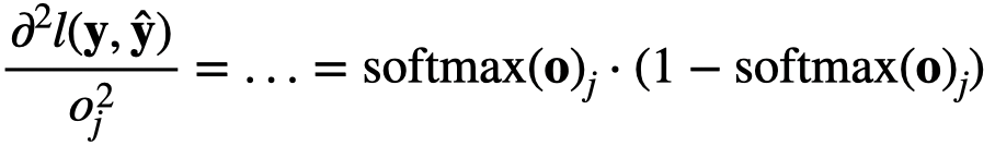
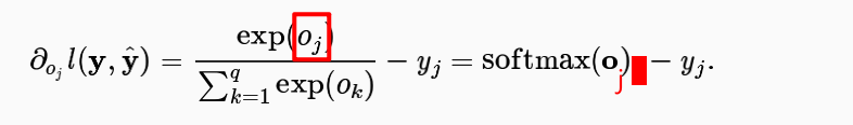
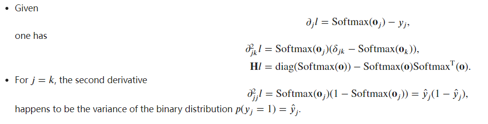
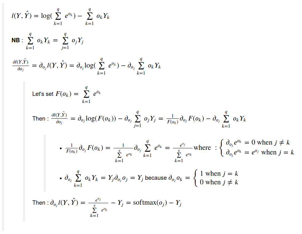
Hi @sheey, the second derivative will be:
$\frac{\partial^2 l(\mathbf{y}, \hat{\mathbf{y}})}{{{o_j^2}}} = … = \mathrm{softmax}(\mathbf{o})_j \cdot (1- \mathrm{softmax}(\mathbf{o})_j)$
i.e.,
Sorry we currently don’t provide the solutions. But feel free to ask question at the discussion forum 
or
When o is vector,j should be outside?
When o_j,j should be in?
We only need to calculate the the derivative of softmax(o)_j (j is in or out?) to get the second derivative of the cross-entropy loss 𝑙(𝐲,𝐲̂) ?
I noticed that the second derivative of the cross-entropy loss 𝑙(𝐲,𝐲̂) is exactly the derivative of softmax(o)_j .
The derivative of y_j is 0 ? y_j is 1 or 0? j represents the label?
Hi @StevenJokes, good question! Actually, $j$ should be outside, since we first calculate softmax of the vector $o$, then take its j’s component.
1 reply
I got it. Thanks @goldpiggy
When we calculate the derivative of $y_j$ is 0, does it mean that we think $y_j$ has no relationship about $o_j$.
1 reply
Hi @StevenJokes, $y_j$ is the real label while $o_j$ is the target, i.e. $y_j$ is not a function of $o_j$.
2 replies
How do we judge whether $a$ is a function of $b$ or not?
Or we just judge by that we haven’t defined it before, rather than whether $a$ has a relationship with $b$ in reality or not.
I think it is a function in reality. But newton’s calculus can’t calculate its derivative, just because the function is discrete.
Please check https://github.com/d2l-ai/d2l-en/issues/1141 quickly, I think it maybe makes all eval wrong.
How do we judge whether $a$ is a function of $b$ or not?
Or we just judge by that we haven’t defined it before, rather than whether $a$ has a relationship with $b$ in reality or not.
Hi @StevenJokes, $y$ is the true label, while $\hat{y}$ is the estimated label. Hence $\hat{y}$ is a function of $o$, while $y$ is not.
1 reply
I already have understand $y_j$ is the true label, such as one-hot. But the diverce of our thinking is that I think the true label has a certain relationship with $o_j$, so I think $y_j$ is also $o_j$'s function. When we get same $o_j$, we get only one and $y_j$. Doesn’t it conform the defination of function.
But the function is discrete.
As we saw in “Freshness and Distribution Shift”, if production data is different from the data a model was trained on, a model may struggle to perform. To help with this, you should check the inputs to your pipeline.
In 10. Build Safeguards for Models - Building Machine Learning Powered Applications [Book]

Although softmax is a nonlinear function, the outputs of softmax regression are still determined by an affine transformation of input features; thus, softmax regression is a linear model.
Can anyone explain this why is it so? because when we say that a model is linear model , then it means model is linear in the parameter but in softmax regression , we are applying softmax function which is non linear so our model parameter will become non linear.
1 reply
Just a statistical speaking!

exercise 1.1

@goldpiggy,
I can’t understand too. 
Hi @Gavin, great question. A simple answer is:
For more details, please check 22.7. Maximum Likelihood — Dive into Deep Learning 1.0.3 documentation
5 replies
@goldpiggy
The simple answer seems to be Tautology.
I have read URL you give.
But I think it didn’t solve this question.
I can’t find anything in it.

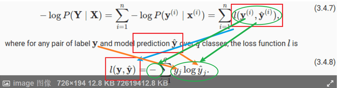
Hello. I am still not able to understand clearly how these 2 equations are related. Can you please explain, how for a particular observation i, the probability y given x is related to the entropy definition overall classes?
Thank you for your response. My question was more specifically why
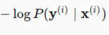 is same as
l(y,y_hat)
Is this because y when 1-hot encoded has only single position with 1 and hence when we sum up the y * log(y_hat) over the entire class, we are left with the probability y_hat corresponding to true y. Please advise.
2 replies
@Abinash_Sahu
l (y,y _ hat)
Cross entropy loss
Only one type of these losses we often use.
https://ml-cheatsheet.readthedocs.io/en/latest/loss_functions.html

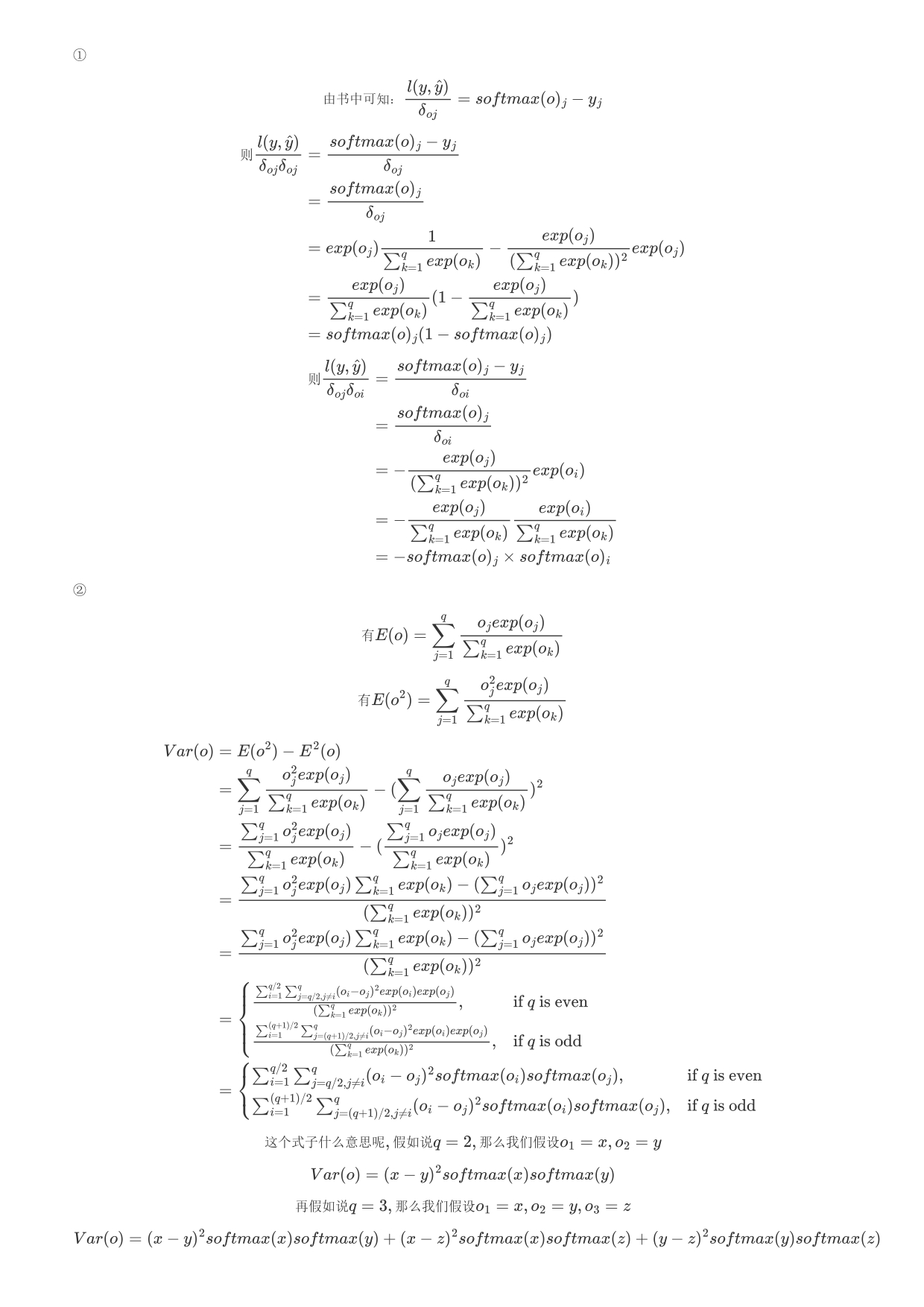
Q1.2. Compute the variance of the distribution given by softmax(𝐨)softmax(o) and show that it matches the second derivative computed above.
Can someone point me in the right direction? I tried to use Var[𝑋]=𝐸[(𝑋−𝐸[𝑋])^2]=𝐸[𝑋^2]−𝐸[𝑋]^2 to find the variance but I ended up having the term 1/q^2… it doesn’t look like the second derivative from Q1.1.
Thanks!
2 replies
It appears that there is a reference that remained unresolved:
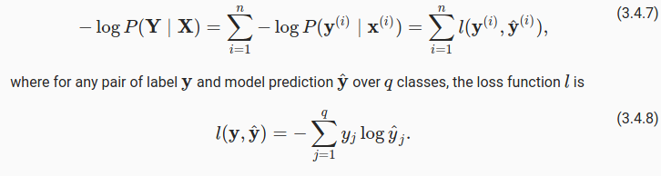
:eqref: eq_l_cross_entropy
in 3.4.5.3
1 reply
Thanks. Now it’s fixed. See comments in https://github.com/d2l-ai/d2l-en/issues/1448

to keep unified form,should the yj in later two equations should have an upper right mark (i) ?


3.1 is strait forward to show.
I’m having trouble with 3.2 and 3.3:
3.2:
Show:
   ⎛   a      b⎞
log⎝𝜆⋅ℯ  + 𝜆⋅ℯ ⎠
──────────────── > Max(a, b)
       𝜆

Assume:
    a > b
    𝜆 > 0

(Max(a,b) -> a, b/c a > b)

   ⎛   a      b⎞
log⎝𝜆⋅ℯ  + 𝜆⋅ℯ ⎠
──────────────── > a
       𝜆

   ⎛   a      b⎞
log⎝𝜆⋅ℯ  + 𝜆⋅ℯ ⎠ > 𝜆a

(exp both sides)

   a      b    𝜆a
𝜆⋅ℯ  + 𝜆⋅ℯ  > ℯ
LHS !> RHS
and 3.3:
I did the calculus and the limit looked like it was going to zero (instead of max(a,b)) so I coded up the function in numpy to check, and indeed it appears to go to 0 instead of 4 in this case (a=2, b=4).
[nav] In [478]: real_softmax = lambda x: 1/x * np.log(x*np.exp(2) + x*np.exp(4))

[ins] In [479]: real_softmax(.1)
Out[479]: 18.24342918048927

[nav] In [480]: real_softmax(1)
Out[480]: 4.126928011042972

[ins] In [481]: real_softmax(10)
Out[481]: 0.6429513104037019

[ins] In [482]: real_softmax(1000)
Out[482]: 0.01103468329002511

[ins] In [483]: real_softmax(100000)
Out[483]: 0.000156398534760132
Please advise
thanks.but i use the definition of variance to derive while your advice is to use inference of variance to do that.both are same in fact
i think you have a mistake at the usage of ∑a/b != ∑a/∑b but ∑a / b as the denominator is public

Hi,
1.1 see 1.2
1.2
import numpy as np
output = np.random.normal(size = (10, 1))
def softmax(output):
denominator = sum(np.exp(output))
return np.exp(output)/denominator
st = softmax(output)
st_2nd = st - st**2
np.var(st)
np.var(st_2nd)
3.1 very simple to prove, just move a or b to left, we prove no matter which one moves to left, we can get [exp(a) + exp(b)]/exp(a) or [exp(a) + exp(b)]/exp(b) and both are greater than 1 so we can prove softmax is larger.

Hi,
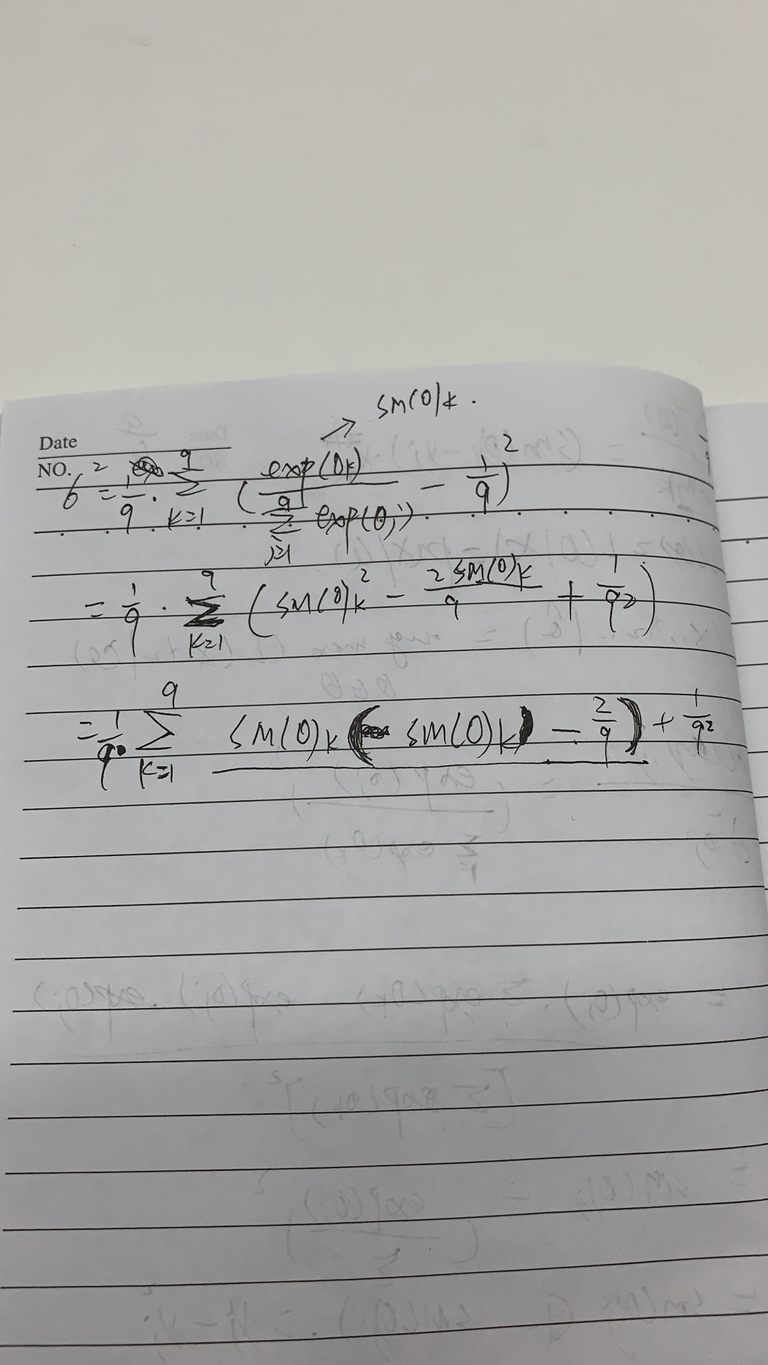
I’m struggling with how the Softmax formula 3.4.9 is re-written (after plugging it in into the loss fct)
I think I understand the first part as you can see from my notes:
https://i.imgur.com/qOq0uuz_d.webp?maxwidth=760&fidelity=grand
However, I struggle to make sense of the lines that come after.
Is the result of 3.4.9 already the derivative, or is it only re-written? And how do they get from 3.4.9 to 3.4.10?
I’m still at the beginning of my DL journey and probably need to freshen up my calculus as well. If someone could point out to me how the formula is transformed that would be great!! I’ve been trying for a while now to write it out, but can’t seem to figure out how it should be done.
this is a great explanation of how the softmax derivative (+ backprop) works which I could follow and understand. But I have problems connecting the solution back to the (more general) formula in 3.4.9
Some help would be much appreciated!
I have the same issue!!
Have you figured it out?
Is the result of 3.4.9 already the derivative, or is it only re-written?
3.4.9 is only the rewritten expression of lost function, not the derivative. It comes mostly from the fact log(a/b) = log(a)-log(b) and that log(exp(X)) = X
And how do they get from 3.4.9 to 3.4.10?
Please check path on the picture here-under

Hi, @goldpiggy,
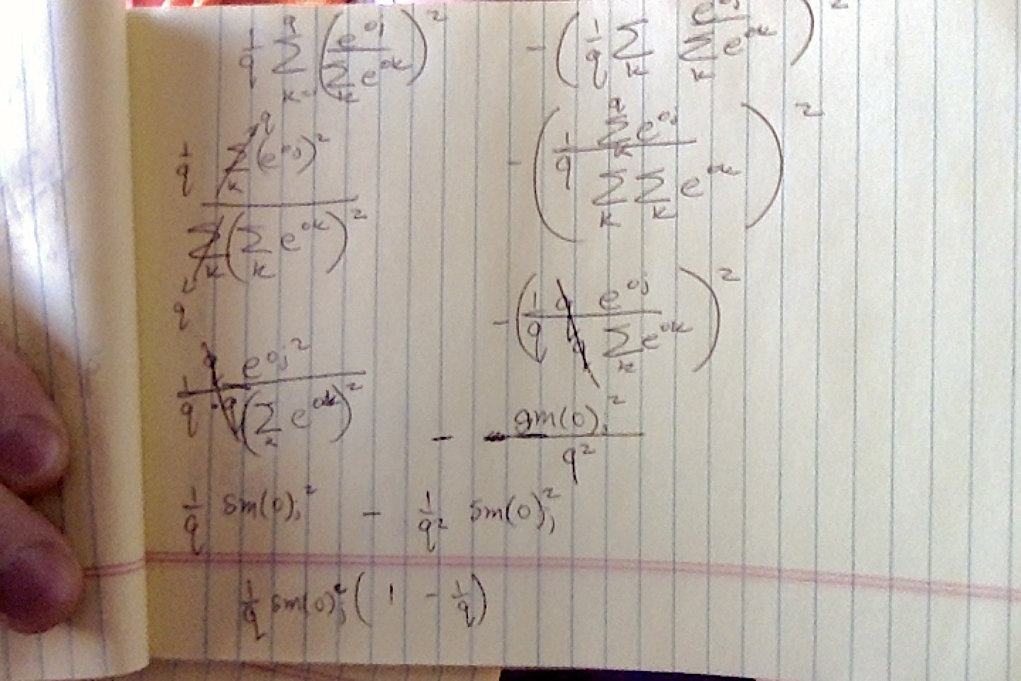
I have a question regarding Excercise 1 of this section of the book. I won’t include details of my calculations in order to keep this as simple as possible. Sorry for my amateurism, but I couldn’t render equations in this box, so I decided to upload them as images. However, because I’m a “new user” I can’t upload more than one image per comment, so I’m posting the rest of this comment as a single image file.

Could you please explain this to me? Thank you in advance for your answer :-).
Great book!
Hey @washiloo, thanks for detailed explanation. Your calculation is almost correct! The reason we are not considering i not equal to j is: you will need to calculate the second order gradient, only when you can explain o_i in some formula by o_j, or it will be zero. There blog here may also help!
Thank you for your reply, @goldpiggy ! However, I don’t understand what do you mean by “only when you can explain o_i in some formula by o_j, or it will be zero”. We are not computing the derivative of o_i with respect to o_j, but the derivative of dl/do_i (wich is a function of all o_i’s) with respect to o_j, and this derivative won’t, in general, be equal to zero. Here, d means “partial derivative” and l is the loss function, but I couldn’t render them properly.
In my early post, I wrote the analytical expression of these second-order derivatives, and you can see that they are zero only when the softmax function is equal to zero for either o_i or o_j, which clearly cannot happen due to the definition of the softmax function.
NOTE: I missed the index 2 for the second-order derivative of the loss function in my early post, sorry.
1 reply
Hi, @goldpiggy. Thank you for your answer.
I think we are talking about different things here. You are talking about the derivatives of o_i w.r.t o_j or the other way around (which are all zero because, as you mention, they are not a function of each other), and I’m talking about the derivatives of the loss function, which depends on all variables o_k (with k = 1,2...,q, because we are assuming that the dimension of 𝐨 is q). We both agree that the gradient of the loss function exists, and this gradient is a q-dimensional vector whose elements are the first-order partial derivatives of the loss function w.r.t. each of the independent variables o_k. Now, each of these derivatives is also a function of all variables o_k, and therefore can be differentiated again to obtain the second-order derivatives, as I explained in my first post. But this is not a problem at all… I understand how to compute these derivatives and I also managed to write a script that computes the Hessian matrix using torch.autograd.grad.
My question is related to Exercise 1 of this section of the book:
“Compute the variance of the distribution given by softmax(𝐨) and show that it matches the second derivative of the loss function.”
As I mentioned before, it is not clear to me what do you mean here by “the second derivative” of the loss function. This “second derivative” should be a real number, because the variance V of the distribution is a real number, and we are trying to show that these quantities are equal. But there are q^2 second-order partial derivatives, so what are we supposed to compare with the variance of the distribution? One of these derivatives? Some function of them?
Thank you in advance for your answer!
3 replies

Does anyone have any idea about Q2? I don’t see the problem about setting the binary code to (1,0,0) (0,1,0) and (0,0,1) on a (1/3, 1/3, 1/3) classification problem. Please reply me if you have any thought on this. Thanks!

@goldpiggy
Hi Goldpiggy,
When we are talking about
as minimizing our surprisal (and thus the number of bits) required to communicate the labels.
in cross-entropy revisited section,
What are we really talking about?
Thank you ![]()

I got the same result as you.I also don’t understand why some discussions assume that the second-order partial derivative equals to variance of softmax when i=j.
Hi @goldpiggy ,
I think in Exercise 3.3, the condition should be \lambda -> positive infinite instead of \lambda->infinite.
Is that right?
Thanks

Sorry guys. here are my wrong answers. I kind of have the feeling that most of this is wrong looking at discussion here. but just putting it here for a sense of completion. But here is my contribution anyway.
depth.
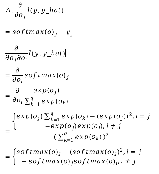
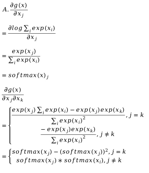
1. Compute the second derivative of the cross-entropy loss l(y, yˆ) for the softmax.
* after applying quotient rule for cross entropy loss the anaswer comes out to be zero.apparentlythis is wrong.
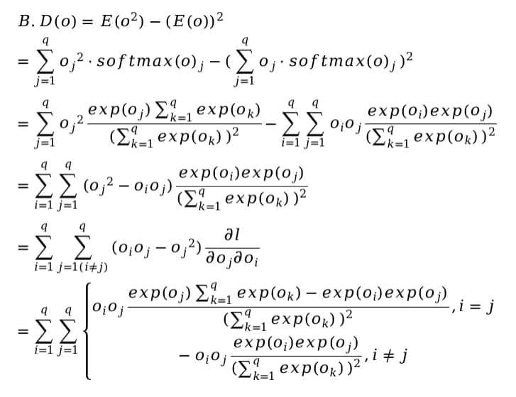
2. Compute the variance of the distribution given by softmax(o) and show that it matches
the second derivative computed above.
* Its close to zero through experiments too. but why should this happen? is second derivative essentially same as variance?
vector is 1/3
1. What is the problem if we try to design a binary code for it?

* We would need at least 2 bits, and 00,01, 10 would be used but not 11. ?

2. Can you design a better code? Hint: what happens if we try to encode two independent
observations? What if we encode n observations jointly?
* we can do it through one hot encoding where the size of array would be the number of observations n
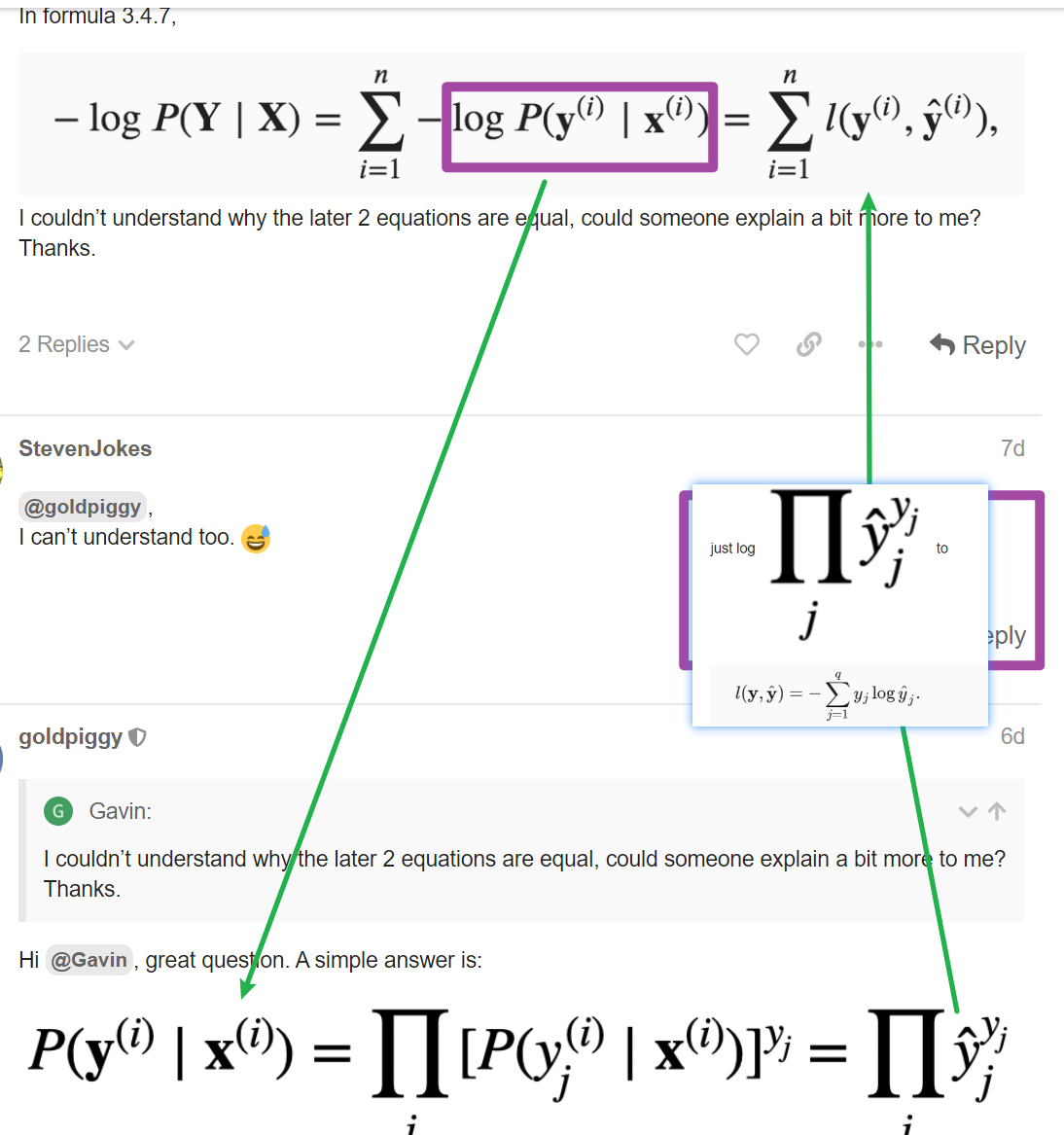
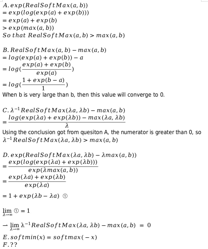
uses it). The real softmax is defined as RealSoftMax(a, b) = log(exp(a) + exp(b)).
1. Prove that RealSoftMax(a, b) > max(a, b).

* verified though not proved
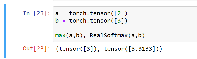
Prove that this holds for λ
−1RealSoftMax(λa, λb), provided that λ > 0.

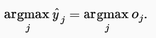
There is a type in the sentence: “Then we can choose the class with the largest output value as our prediction…” it should be y hat at in the argmax rather than y

I’ve got the same result for the second derivative of the loss but I don’t know how to compute the variance or how it relates with the second derivative.
Did you make any progress ?

Hello,
I have the following error which I cannot seem to resolve. Can anyone help me out? Thanks


Think about the relationship between Hessian Matrix and Covariance Matrix

I think because the y in this equation 3.4.10 is an one_hot vector. so the sum of y_js is equal to y_j of the correct label.

I am unsure what this question is trying to get at:
- Assume that we have three classes which occur with equal probability, i.e., the probability vector is (1/3,1/3,1/3).
- What is the problem if we try to design a binary code for it?
- Can you design a better code? Hint: what happens if we try to encode two independent observations? What if we encode n observations jointly?
My guess is simply that binary encoding doesn’t work when you have more than 2 categories, and one hot encoding with possibilities (1,0,0), (0,1,0) and (0,0,1) works better.
However, this doesn’t seem to address the specific probability or the hint given, so I think my guess is too simplistic.
Any further reading suggestion for question 7?

Here are my opinions for the exs:
I still not sure about ex.1, ex.5.E, ex.5.F, ex.6
ex.1
ex.2
A. If I use binary code for the three class, like 00, 01, 11, then the distance between 00 and 01 is smaller than that between 00 and 11, that is oppose to the fact that the three class is of equal probability.
B. I think I should use one-hot coding mentioned in this chapter, because for any independent observation(which I think is a class), there contains no distance information between any pair of them.
ex.3
Two ternaries can have 9 different representation, so my answer is 2.
This ternary is suitable for electronics because in a physical wire, there will be three distinctive condition: positive voltage, negative voltage, zero voltage.
ex.4
A. Bradley-Terry model is like
![]()
When there are only two classes, softmax just fit this.
B. No matter how many classes there will be, if I put a higher score for class A compared to class B, the the B-T model will still let me chose class A, and after 3 times of comparing, I will chose the class with the highest score, that still holds true for the softmax.
ex.5
ex.6
This is my procedure for question A, but I can’t prove that the second derivative is just the variance.
ex.7
A. Because of exp(−𝐸/𝑘𝑇), if I double T, alpha will go to 1/2, and if I halve it, alpha will go to 2, so T and alpha goes in opposite direction.
B. If T converge to 0, the possibility for any class will converge to 0, and the proportion between two class i and j exp( -(Ei - Ej) /kT) will also converge to 0. Like a frozen object of which all molecules is static.
C. If T converge to ∞, the proportion between two class i and j will converge to 1, which means every class has the same possibility to show up.

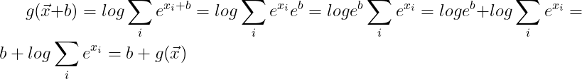
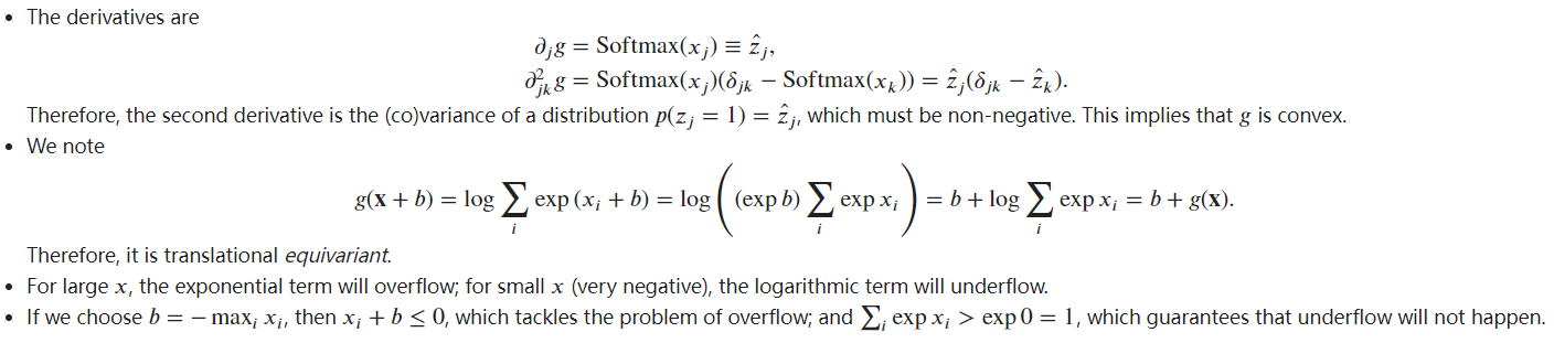
Exercise 6 Show that g(x) is translation invariant, i.e., g(x+b) = g(x)
I don’t see how this can be true for b different from 0.


Ex1.
Ex6 (issue: (1) translational invariant or equivariant? (Softmax is invariant, but log-sum-exp should be equivariant); (2) b or negative b? Adding maximum can make overflow problem worse).

To ex.1, maybe we can take softmax distribution as Bernoulli distribution with a probability of $p = softmax(o)$, so the variance is:
$$Var[X] = E[X^2] - E[X]^2 = \text{softmax}(o)(1 - \text{softmax}(o))$$
I don’t know whether this suppose is right
and my solutions to the exs: 4.1

Does this mean that each coordinate of each y label vector is independent of each other? Also, shouldn’t the y_j of the last 2 equations also have a “i” superscript?
I read the URL given, but it doesn’t clarify too much for this specific case.

could this equation be generalized if $\textbf{y^{i}}$ was not one-hot encoded vector but a soft label or a probability distribution?
1 reply
I think here should be the author wanted to express.
P=\prod{ P(\vec{y}{i}|\vec{x} {i}) }
\vec{x}{i} is the i th image, is the a 4X1 vector in case of a 2x2 image
\vec{y} {i} is the softmax result, is a 3X1 vector in case of 3 different classification results.
The P means we must max the accuracy of all the n image classification results, not only a single image. Am I correct?
how ever, the result P should be a 3X1 vector eventually.
The superscript $i$ indicates the i-th data sample and its corresponding label. And in the context of image classification here, yes, $\textbf{x}^{(i)}$ is the pixel tensor that represents the i-th image, $\textbf{y}^{(i)}$ is the category vector of this image.
What I asked is that if or not this equation could be applied to a general case, namely $\textbf{y}^{(i)}$ is not a one-hot encoded vector but a vector presents possibilities for each category. In my understanding after reading section 22.7, the answer is no.

In any exponential family model, the gradients of the log-likelihood are given by precisely this term. This fact makes computing gradients easy in practice.
I’m confused by this statement because it claims that the gradient of log likelihood w.r.t. the outputs (which is Xw+b) is y_hat-y, for any exponential family distribution. Poisson distribution belongs to this family, but y_hat-y would be an integer, while the gradient can be any real number.
Q6

 ?
?