Looks like you have der(E[X]^2), but what about E[X^2]? Recall:
Var[X] = E[X^2] - E[X]^2
3.1 is strait forward to show.
I’m having trouble with 3.2 and 3.3:
3.2:
Show:
   ⎛   a      b⎞
log⎝𝜆⋅ℯ  + 𝜆⋅ℯ ⎠
──────────────── > Max(a, b)
       𝜆

Assume:
    a > b
    𝜆 > 0

(Max(a,b) -> a, b/c a > b)

   ⎛   a      b⎞
log⎝𝜆⋅ℯ  + 𝜆⋅ℯ ⎠
──────────────── > a
       𝜆

   ⎛   a      b⎞
log⎝𝜆⋅ℯ  + 𝜆⋅ℯ ⎠ > 𝜆a

(exp both sides)

   a      b    𝜆a
𝜆⋅ℯ  + 𝜆⋅ℯ  > ℯ
LHS !> RHS
and 3.3:
I did the calculus and the limit looked like it was going to zero (instead of max(a,b)) so I coded up the function in numpy to check, and indeed it appears to go to 0 instead of 4 in this case (a=2, b=4).
[nav] In [478]: real_softmax = lambda x: 1/x * np.log(x*np.exp(2) + x*np.exp(4))

[ins] In [479]: real_softmax(.1)
Out[479]: 18.24342918048927

[nav] In [480]: real_softmax(1)
Out[480]: 4.126928011042972

[ins] In [481]: real_softmax(10)
Out[481]: 0.6429513104037019

[ins] In [482]: real_softmax(1000)
Out[482]: 0.01103468329002511

[ins] In [483]: real_softmax(100000)
Out[483]: 0.000156398534760132
Please advise
thanks.but i use the definition of variance to derive while your advice is to use inference of variance to do that.both are same in fact
i think you have a mistake at the usage of ∑a/b != ∑a/∑b but ∑a / b as the denominator is public
2 Likes
Hi,
1.1 see 1.2
1.2
import numpy as np
output = np.random.normal(size = (10, 1))
def softmax(output):
denominator = sum(np.exp(output))
return np.exp(output)/denominator
st = softmax(output)
st_2nd = st - st**2
np.var(st)
np.var(st_2nd)
3.1 very simple to prove, just move a or b to left, we prove no matter which one moves to left, we can get [exp(a) + exp(b)]/exp(a) or [exp(a) + exp(b)]/exp(b) and both are greater than 1 so we can prove softmax is larger.
Hi,
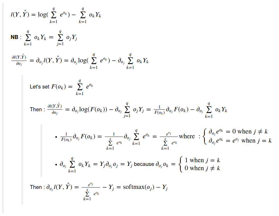
I’m struggling with how the Softmax formula 3.4.9 is re-written (after plugging it in into the loss fct)
I think I understand the first part as you can see from my notes:
https://i.imgur.com/qOq0uuz_d.webp?maxwidth=760&fidelity=grand
However, I struggle to make sense of the lines that come after.
Is the result of 3.4.9 already the derivative, or is it only re-written? And how do they get from 3.4.9 to 3.4.10?
I’m still at the beginning of my DL journey and probably need to freshen up my calculus as well. If someone could point out to me how the formula is transformed that would be great!! I’ve been trying for a while now to write it out, but can’t seem to figure out how it should be done.
this is a great explanation of how the softmax derivative (+ backprop) works which I could follow and understand. But I have problems connecting the solution back to the (more general) formula in 3.4.9
Some help would be much appreciated! 
I have the same issue!!
Have you figured it out?
Is the result of 3.4.9 already the derivative, or is it only re-written?
3.4.9 is only the rewritten expression of lost function, not the derivative. It comes mostly from the fact log(a/b) = log(a)-log(b) and that log(exp(X)) = X
And how do they get from 3.4.9 to 3.4.10?
Please check path on the picture here-under
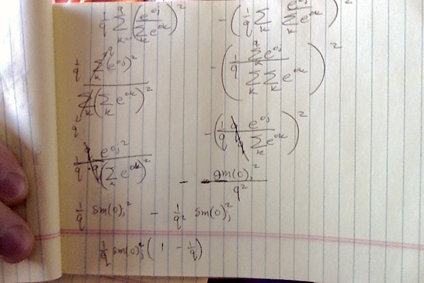
Hi, @goldpiggy,
I have a question regarding Excercise 1 of this section of the book. I won’t include details of my calculations in order to keep this as simple as possible. Sorry for my amateurism, but I couldn’t render equations in this box, so I decided to upload them as images. However, because I’m a “new user” I can’t upload more than one image per comment, so I’m posting the rest of this comment as a single image file.

Could you please explain this to me? Thank you in advance for your answer :-).
Great book!
Hey @washiloo, thanks for detailed explanation. Your calculation is almost correct! The reason we are not considering i not equal to j is: you will need to calculate the second order gradient, only when you can explain o_i in some formula by o_j, or it will be zero. There blog here may also help!
Thank you for your reply, @goldpiggy ! However, I don’t understand what do you mean by “only when you can explain o_i in some formula by o_j, or it will be zero”. We are not computing the derivative of o_i with respect to o_j, but the derivative of dl/do_i (wich is a function of all o_i’s) with respect to o_j, and this derivative won’t, in general, be equal to zero. Here, d means “partial derivative” and l is the loss function, but I couldn’t render them properly.
In my early post, I wrote the analytical expression of these second-order derivatives, and you can see that they are zero only when the softmax function is equal to zero for either o_i or o_j, which clearly cannot happen due to the definition of the softmax function.
NOTE: I missed the index 2 for the second-order derivative of the loss function in my early post, sorry.
Hey @washiloo, first be aware that o_j and o_i are independent observations. i.e., o_i cannot be explained by a function of o_j. If there are independent, the derivatives will be zero. Does this helps?
Hi, @goldpiggy. Thank you for your answer.
I think we are talking about different things here. You are talking about the derivatives of o_i w.r.t o_j or the other way around (which are all zero because, as you mention, they are not a function of each other), and I’m talking about the derivatives of the loss function, which depends on all variables o_k (with k = 1,2...,q, because we are assuming that the dimension of 𝐨 is q). We both agree that the gradient of the loss function exists, and this gradient is a q-dimensional vector whose elements are the first-order partial derivatives of the loss function w.r.t. each of the independent variables o_k. Now, each of these derivatives is also a function of all variables o_k, and therefore can be differentiated again to obtain the second-order derivatives, as I explained in my first post. But this is not a problem at all… I understand how to compute these derivatives and I also managed to write a script that computes the Hessian matrix using torch.autograd.grad.
My question is related to Exercise 1 of this section of the book:
“Compute the variance of the distribution given by softmax(𝐨) and show that it matches the second derivative of the loss function.”
As I mentioned before, it is not clear to me what do you mean here by “the second derivative” of the loss function. This “second derivative” should be a real number, because the variance V of the distribution is a real number, and we are trying to show that these quantities are equal. But there are q^2 second-order partial derivatives, so what are we supposed to compare with the variance of the distribution? One of these derivatives? Some function of them?
Thank you in advance for your answer!
In formula (3.4.10):
Why the derivative in the second term is y_j and not the sum(y_j) ?. Can somebody explain me?
Thanks
Does anyone have any idea about Q2? I don’t see the problem about setting the binary code to (1,0,0) (0,1,0) and (0,0,1) on a (1/3, 1/3, 1/3) classification problem. Please reply me if you have any thought on this. Thanks!
@goldpiggy
Hi Goldpiggy,
When we are talking about
as minimizing our surprisal (and thus the number of bits) required to communicate the labels.
in cross-entropy revisited section,
What are we really talking about?
Thank you ![]()
I got the same result as you.I also don’t understand why some discussions assume that the second-order partial derivative equals to variance of softmax when i=j.
Hi @goldpiggy ,
I think in Exercise 3.3, the condition should be \lambda -> positive infinite instead of \lambda->infinite.
Is that right?
Thanks