I noticed that 2.5.2 does’t have PyTorch, so I tried to convert it.
I used “.detach()” and “.clone()” to simulate “.copy()” in MXNET.
But I’m confused with differences from “.detach()” and “.clone()”.
Which one is more like to “.copy()” in MXNET?
from torch.autograd import Variable

x = torch.arange(4.0, requires_grad=True)

# make it as a Variable with a gradient taken.

x =  torch.autograd.Variable(x, requires_grad=True)

y = x * x

y.backward(torch.ones(y.size()))
AttributeError: ‘Tensor’ object has no attribute ‘copy’
# detach

u = x.detach()

# replace :u = torch.autograd.Variable(u, requires_grad=True)

# make tensor autograd works

u.requires_grad()

v = u * u

v.backward(torch.ones(v.size()))

x.grad == u.grad
tensor([True, True, True, True])
# clone

u = x.clone()

u.requires_grad()

v = u * u

v.backward(torch.ones(v.size()))

x.grad == u.grad
“Consequently d / a allows us to verify that the gradient is correct.”
I didn’t understand the meaning of d / a.
So I code as follow. But now, I’m more confused.
b = torch.randn(size=(1,), requires_grad=True)
b = b + 1000
# record the calculation
d = f(b)
d.backward()
b.grad == (d / b)
False
d tensor([1999.6416], grad_fn=) b tensor([999.8208], grad_fn=)
t = b.grad
t
no return?
2.5.5.
The MXnet code of prediction mode haven’t mentioned.
I was wondering about the PyTorch’s code.
I’m not very clear. Maybe second derivative is more easy to overflow the scope of storages.
y.backward()
RuntimeError: Trying to backward through the graph a second time, but the buffers have already been freed. Specify retain_graph=True when calling backward the first time.
y = 2 * torch.dot(x, x)

y

y.backward(retain_graph=True)

y.backward(retain_graph=True)
no Error!
Error happened!
# matrix

a = torch.randn(20, requires_grad=True).reshape(5, 4)

d = f(a)

d.backward()
RuntimeError: grad can be implicitly created only for scalar outputs
analyze:
source code:~.conda\envs\pytorch\lib\site-packages\torch\autograd_init_.py in _make_grads(outputs, grads)
rows:from 32 to 35 :
        elif grad is None: # why grad is None? Does f(a) not support matrix?

            if out.requires_grad:

                if out.numel() != 1:

                    raise RuntimeError("grad can be implicitly created only for scalar outputs")
TODO:
I’m trying to import plot in 2.4, so I convert the “2-4.ipynb” to “two-four.py”.
But when I import it, it just happens as follow. How to fix it?
from ..d2l import torch as d2l

from IPython import display

import numpy as np

from .two_four import plot
ImportError Traceback (most recent call last)
in
----> 1 from …d2l import torch as d2l
  2 from IPython import display

  3 import numpy as np

  4 from .two_four import plot
ImportError: attempted relative import with no known parent package
Can you explain what exactly is the doubt here?
To import -> from d2l import torch as d2l you first need to install the d2l package in your environment.
The first reply is my 2.5.2’s pytorch code. I use “detach” and “clone” to simulate what “copy” do in MXNET. But which one is best, “detach” or “clone”?
The second reply is about "the meaning of d / a " in 2.5.4. I tried another “b”.The return of “b.grad == (d / b)” is false rather than true. why?
The third reply is my answer to 2.5.7. I’m still working on how to import plot in 2.4.
After running pip install -U d2l -f https://d2l.ai/whl.html,
I can directly run from d2l import torch as d2l
Thanks
But I’m confused about the bug when I directly run the imtorch.py(rename from d2l/torch.py)
$ /usr/bin/env python "d:\onedrive\文档\read\d2l\d2l\imtorch.py"
Traceback (most recent call last):
  File "d:\onedrive\文档\read\d2l\d2l\imtorch.py", line 22, in <module>
    import torch
  File "C:\ProgramData\Anaconda3\lib\site-packages\torch\__init__.py", line 81, in <module>
    ctypes.CDLL(dll)
  File "C:\ProgramData\Anaconda3\lib\ctypes\__init__.py", line 364, in __init__
    self._handle = _dlopen(self._name, mode)
OSError: [WinError 126] The specified module could not be found
Answer to first question. tensor.detach() creates a tensor that shares the same storage with tensor that does not require grad.
But tensor.clone() will also give you original tensor’s requires_grad attributes. It is basically an exact copy including the computation graph.
Use detach() to remove a tensor from computation graph and use clone to copy the tensor while still keeping the copy as a part of the computation graph it came from.
The second answer about "the meaning of d / a " in 2.5.4.
“a.grad == (d / a)” is true because if you see how d is calculate using f(a). It is basically scaling a by some constant factor k. And if you were to do differentiate such a function say function d=k*a with respect to a then you would get that k. Hence these are true and obviously it won’t hold for b because d is a function of which scales a and not b.
Answer to third question.
As i suggested earlier and you probably did it, you can simply pip install d2l to import torch from d2l.
If you want to import the specific rename imtorch.py just add this to the start of your code before making the import. ->
Q1.
Does it mean that if I ‘clone’ a tensor or a Variable that has requires_grad attribute, then I don’t need to .requires_grad() for the new one?
Use detach() to remove a tensor? However, why can I still judge x.grad() == u.grad? “Remove” doesn’t mean that x will not exist? I think that x and u are just two different names for the same storage.
Can my code about 2.5.2’s Variable add to 2.5.2?
Q2.
I have understand that d is a function of which scales a. But what difference with f(b)?
Because, I think that f(b) = 2 * b.
First, b(formal parameter) =2 * a (argument b).
Then, not enter the loop. (b > 1000)
Then, True for if, return b(formal parameter) which is 2 * b(argument)
Q3.
Thanks. I will try it next time. I have did pip install d2l The specified module could not be found
Did the problem happen because the module doesn’t exist in my sys.path?
import numpy as np
from d2l import torch as d2l
x = np.linspace(- np.pi,np.pi,100)
x = torch.tensor(x, requires_grad=True)
y = torch.sin(x)
for i in range(100):
y[i].backward(retain_graph = True)
d2l.plot(x.detach(),(y.detach(),x.grad),legend = ((‘sin(x)’,“grad w.s.t x”)))
looks dummy since I compute the grad 100 times, is there any better way?
My understanding is that by default the framework will convert the actual output matrix into a vector based on a “gradient vector” that we passed in. The description of this “gradient vector” is
which specifies the gradient of the differentiated function w.r.t self.
What does it mean? Does “gradient of differentiated function” mean “second order gradient”?
My answers to the questions: please point out if I am misunderstood anything
Why is the second derivative much more expensive to compute than the first derivative?
Because instead of following the original computation graph, we need to construct a new one that corresponds to the calculation of first-order gradient?
After running the function for backpropagation, immediately run it again and see what happens.
RuntimeError: Trying to backward through the graph a second time, but the saved intermediate results have already been freed. Specify retain_graph=True when calling backward the first time.
In the control flow example where we calculate the derivative of d with respect to a , what would happen if we changed the variable a to a random vector or matrix. At this point, the result of the calculation f(a) is no longer a scalar. What happens to the result? How do we analyze this?
Directly changing would give the “blah blah … only scalar output” which is what 2.5.2 is talking about. I changed the code to
a = torch.randn(size=(3,), requires_grad=True)
d = f(a)
d.sum().backward()
and a.grad == d / a still gives true. This is because in the function, there is no cross-element operation. So each element of the vector is independent and doesn’t affect other element’s differentiation.
Redesign an example of finding the gradient of the control flow. Run and analyze the result.
SKIP
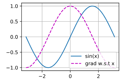
Let $f(x) = \sin(x)$. Plot $f(x)$ and $\frac{df(x)}{dx}$, where the latter is computed without exploiting that $f’(x) = \cos(x)$.
import numpy as np
from d2l import torch as d2l
x = np.linspace(- np.pi,np.pi,100)
x = torch.tensor(x, requires_grad=True)
y = torch.sin(x)
y.sum().backward()

d2l.plot(x.detach(),(y.detach(),x.grad),legend = (('sin(x)',"grad w.s.t x")))
Hi, May I confirm my understanding about the auto differentiation of Python control flow?
I assume, as long as the Python control flow is established by functions and variables from Pytorch, then the auto differentiation is doable. Am I right on this? No other functions should be involved such as sin() from math package(have to use sin() from Pytorch instead if I want auto differentiation).
Exercise 1. The second derivative is much more expensive because, for a function f with n variables, the Hessian Matrix has n² elements while the gradient vector has n elements. In other words, there are n² possible second order derivatives ( ∂²f/∂x1², ∂²f/∂x1∂x2, …) while there are n possible first order derivatives (∂f/∂x1, ∂f/∂x2, …, ∂f/∂xn).
Seems, in the text, by calculating y.backward(torch.ones(len(x))), we contract the Jacobian over the 4 components of y(x). The Jacobian is a 4x4 matrix. I can extract each column via y.backward(torch.tensor([1,0,0,0])), #where i shift the 1 to each of the 4 column slots.
Is this best way to calculate the Jacobian?
My anwser for ex 2 3 4,welcom to tell me if you find any error
'''
ex.2
Aafter running the function for backpropagation, immediately run it again and see what hap-
pens. Why?

reference:
[https://blog.csdn.net/rothschild666/article/details/124170794](https://blog.csdn.net/rothschild666/article/details/124170794)
'''
import torch
x = torch.arange(4.0, requires_grad=True)
x.requires_grad_(True)
y = 2 * torch.dot(x, x)
y.backward(retain_graph=True)#need to set para = Ture
y.backward()
x.grad
out for ex2:
tensor([ 0., 8., 16., 24.])
'''
ex.3
In the control flow example where we calculate the derivative of d with respect to a, what
would happen if we changed the variable a to a random vector or a matrix? At this point, the
result of the calculation f(a) is no longer a scalar. What happens to the result? How do we
analyze this?


reference:
[https://www.jb51.net/article/211983.htm](https://www.jb51.net/article/211983.htm)
'''
import torch
def f(a):
    b = a * 2
    while b.norm() < 1000:
        b = b * 2
    if b.sum() > 0:
        c = b
    else:
        c = 100 * b
    return c
a = torch.randn(size=(2,3), requires_grad=True)
#a = torch.tensor([1.0,2.0], requires_grad=True)
print(a)
d = f(a)
d.backward(d.detach())#This is neccesary, I don't know why, is it because there are b and c in the function?
#d.backward()#wrong
print(a.grad)
out for ex3:
tensor([[-0.6848, 0.2447, 1.5633],
[-0.1291, 0.2607, 0.9181]], requires_grad=True)
tensor([[-179512.9062, 64147.3203, 409814.3750],
[ -33844.5430, 68346.7969, 240686.7344]])
'''
ex.4
Let f (x) = sin(x). Plot the graph of f and of its derivative f ′ . Do not exploit the fact that
f ′ (x) = cos(x) but rather use automatic differentiation to get the result.
'''
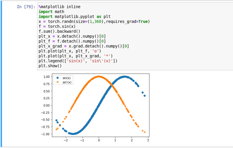
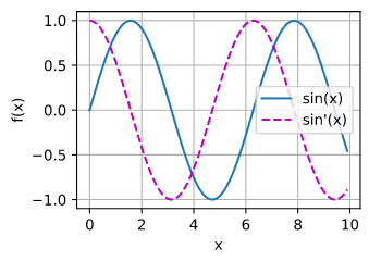
#suppose the functions in 2.4.2Visualization Utilities has been constructed in d2l
from d2l import torch as d2l
x = d2l.arange(0,10,0.1, requires_grad = True)
y = d2l.sin(x)
y.backward(gradient=d2l.ones(len(y)))#y.sum().backward() can do the same thing
#.detach.numpy() is needed because x is set to requires_grad = True
d2l.plot(x.detach().numpy(), [y.detach().numpy(),x.grad], 'x', 'f(x)', legend = ['sin(x)','sin\'(x)'])
Can someone please explain the result of 2.5.1 to me. I understand how the first function is just y = 2x^2, but creating the new function that is y = x.sum(), just returns 6. Is this conceptually 6x or is it just 6 or is this just x (i’m assuming the third because that’s the only way we can get 1 as the gradient all the time) or am i missing something?
My understanding about 2.5.1’s pytorch code blocks:
y = x.sum() is just a way of defining a computational graph in PyTorch, which means evaluating each component of x and adding them up. Gradients are computed on each component of x, NOT on the y graph. Evaluating gradient on a component of x means computing for y_i = x_i (which yields 1).
The same principal applies to the y = 2 * x^Tx part, y is NOT 2x^2, it’s a computational graph for evaluating 2 * x^Tx where each component of it is actually y_i = 2 * x_i * x_i. So the graph y is in fact sum { 2 * x_i * x_i }.
Can someone help with Questions 5 and 6. Is this a pen-paper question, writing down backprop for the computation graph, or is this supposed to be implemented (if yes, then can someone elaborate more on it or provide a solution.)
Also problems 7, 8 are difficult ones, but at least there is a good resource provided by Denis Kazakov.
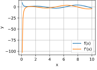
Hi! In Exercise 5, I don’t understand why my solution and the expected derivative do not correspond:
%matplotlib inline
import numpy as np
from matplotlib_inline import backend_inline
from d2l import torch as d2l
import math
x = torch.linspace(0.1, 10, 100)
x.requires_grad_(True)
def f(x):
return ((torch.log(x ** 2)) * torch.sin(x)) + (x ** -1)
y = f(x)
y.backward(torch.ones_like(y))
p = x.grad
Plot the function and its derivative
plt.plot(x.detach().numpy(), y.detach().numpy(), label=‘f(x)’)
plt.plot(x.detach().numpy(), p.detach().numpy(), label=“f’(x)”)
plt.xlabel(‘x’)
plt.ylabel(‘y’)
plt.legend()
plt.grid(True)
plt.show()
gives me this plot:
and when I compare
desired_derivative = -(2 / x) * torch.sin(x) + torch.log(x**2) * torch.cos(x) - (1/x **2)
p == desired_derivative
it evaluates to False.
Can you help me?
import torch
x = torch.arange(4.0)
x.requires_grad_(True)
y = x @ x
y.backward()
Output (second run):
---------------------------------------------------------------------------
RuntimeError                              Traceback (most recent call last)
/tmp/ipykernel_82/1055444503.py in <module>
----> 1 y.backward()

/opt/miniconda/lib/python3.7/site-packages/torch/_tensor.py in backward(self, gradient, retain_graph, create_graph, inputs)
    394                 create_graph=create_graph,
    395                 inputs=inputs)
--> 396         torch.autograd.backward(self, gradient, retain_graph, create_graph, inputs=inputs)
    397
    398     def register_hook(self, hook):

/opt/miniconda/lib/python3.7/site-packages/torch/autograd/__init__.py in backward(tensors, grad_tensors, retain_graph, create_graph, grad_variables, inputs)
    173     Variable._execution_engine.run_backward(  # Calls into the C++ engine to run the backward pass
    174         tensors, grad_tensors_, retain_graph, create_graph, inputs,
--> 175         allow_unreachable=True, accumulate_grad=True)  # Calls into the C++ engine to run the backward pass
    176
    177 def grad(

RuntimeError: Trying to backward through the graph a second time (or directly access saved tensors after they have already been freed). Saved intermediate values of the graph are freed when you call .backward() or autograd.grad(). Specify retain_graph=True if you need to backward through the graph a second time or if you need to access saved tensors after calling backward.
The .backward() call will automatically free all the intermediate tensors in a computational graph after the backprop.
In that sense, “double backward” can not be realized unless one specifies retain_graph=True.
Ex3.
def f(a):
    b = a * 2
    while b.norm() < 1000:
        b = b * 2
    if b.sum() > 0:
        c = b
    else:
        c = 100 * b
    return c
a = torch.randn(size=(4, ), requires_grad=True)
d = f(a)
d.backward()
Output:
---------------------------------------------------------------------------
RuntimeError                              Traceback (most recent call last)
/tmp/ipykernel_82/535593037.py in <module>
      1 a = torch.randn(size=(4, ), requires_grad=True)
      2 d = f(a)
----> 3 d.backward()

/opt/miniconda/lib/python3.7/site-packages/torch/_tensor.py in backward(self, gradient, retain_graph, create_graph, inputs)
    394                 create_graph=create_graph,
    395                 inputs=inputs)
--> 396         torch.autograd.backward(self, gradient, retain_graph, create_graph, inputs=inputs)
    397
    398     def register_hook(self, hook):

/opt/miniconda/lib/python3.7/site-packages/torch/autograd/__init__.py in backward(tensors, grad_tensors, retain_graph, create_graph, grad_variables, inputs)
    164
    165     grad_tensors_ = _tensor_or_tensors_to_tuple(grad_tensors, len(tensors))
--> 166     grad_tensors_ = _make_grads(tensors, grad_tensors_, is_grads_batched=False)
    167     if retain_graph is None:
    168         retain_graph = create_graph

/opt/miniconda/lib/python3.7/site-packages/torch/autograd/__init__.py in _make_grads(outputs, grads, is_grads_batched)
     65             if out.requires_grad:
     66                 if out.numel() != 1:
---> 67                     raise RuntimeError("grad can be implicitly created only for scalar outputs")
     68                 new_grads.append(torch.ones_like(out, memory_format=torch.preserve_format))
     69             else:

RuntimeError: grad can be implicitly created only for scalar outputs
Since a as well as d is no longer a scalar, we need to reduce d to make backprop feasible.
d.sum().backward()
a.grad == d / a
Output:
tensor([True, True, True, True])
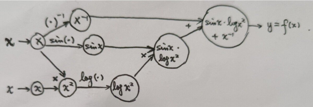
Ex4-5.
The dependency graph (computational graph):
Applying the backprop algorithm according to the chain rule…
The + operation y = n1 + n2: n1.grad = 1, n2.grad = 1
The inverse operation n1 = 1 / x: x.grad1 = (- 1 / x ** 2) * n1.grad = - 1 / x ** 2
I’m probably too late for you, but posting here for posterity.
Firstly, you need to use torch.log10(x**2) in your f(x) function, as just “log” function is for natural logarithm, and we’re given “log base 10” in question. And for the same reason I guess, you’ve mistakenly calculated derivative considering natural log of x squared. I’m leaving the code below with correct derivative.
You might get some “False” values when comparing AD and desired derivative results, but those are just because of unreliable floating point math of computers.
Assuming we’re talking about the derivative of a scalar with respect to a tensor, the first derivative will be of the same size as the tensor. But the second derivative will be of that size, squared! Further, autodiff only requires a single backward pass to find the gradients - but if we want to find the full Hessian, we then need to find the derivative of each component of our initial gradients. So you’d have to a full backwards pass for every parameter, or find a more efficient way of computing this.
When you run .backward() multiple times, the gradients accumulate (are added to each other).
The shape of f(a) will match the shape of a, so if a is a vector or matrix, we’ll need to call something like .sum().backward() or .backward(torch.ones_like(d)). Once we do, a.grad == d / a will yield a tensor of the same shape as a, with all True values.
See the code below:
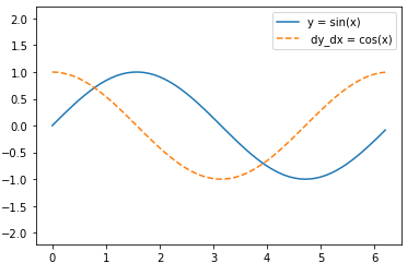
import torch
import matplotlib.pyplot as plt
x = torch.linspace(-5, 5, 100, requires_grad=True)
y = torch.sin(x)
y.sum().backward()
plt.plot(x.detach(), y.detach())
plt.plot(x.detach(), x.grad.detach())
plt.legend(["sin(x)", "dy/dx sin(x)"])
print((x.grad == torch.cos(x)).all())
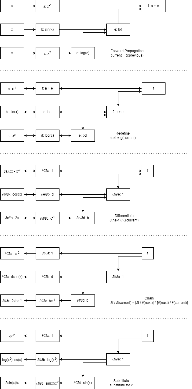
Questions 5-7
I did these on paper by hand. For anyone having a hard time with questions 5-7, I recommend working through this tutorial from Andrej Karpathy.
Question 8
I tried doing forwardprop by hand on a number of computational graphs. For each input, one has to perform a full forward pass through the graph. In contexts where we’d like to track the gradient of some output with respect to one or a few specific inputs, forwardprop makes sense! It would also make sense in any context where we have N inputs and M outputs, and N << M. In practice, neural networks have a massive number of inputs and a scalar output loss, making backwards differentiation the obvious choice. A rule of thumb is that the forward-mode cost is proportional to the number of inputs, and the backward-mode cost is proportional to the number of outputs.
Other tradeoffs may come up in practice, depending on the layout of your computational graph. For example, backprop starts off at a scalar, and the computational graph fans out from there. You might think this makes it difficult to parallelize early parts of the graph, but in practice, backprop parallelizes very well. One might think that forwardprop would be easier to parallelize (since you can start out propogating from all inputs in parallel), but you could get weird dependency bottlenecks as different branches have to be “merged” deeper into the network: if branch A from input a and branch B from input b must be multiplied together, and branch A is very fast to propogate through but branch B is very slow to propogate through, branch A will be bottlenecked by branch B. Generally, you’ll be bottlenecked by the slowest path through the network.
Another tradeoff is memory usage: backprop requires storing intermediate activations from the forward pass, meaning memory usage scales with the depth of a network. Forwardprop doesn’t have this requirement! Aside from tracking the partial derivatives at each step, forwardprop stateless as we move through the network, meaning the memory footprint is generally much smaller.
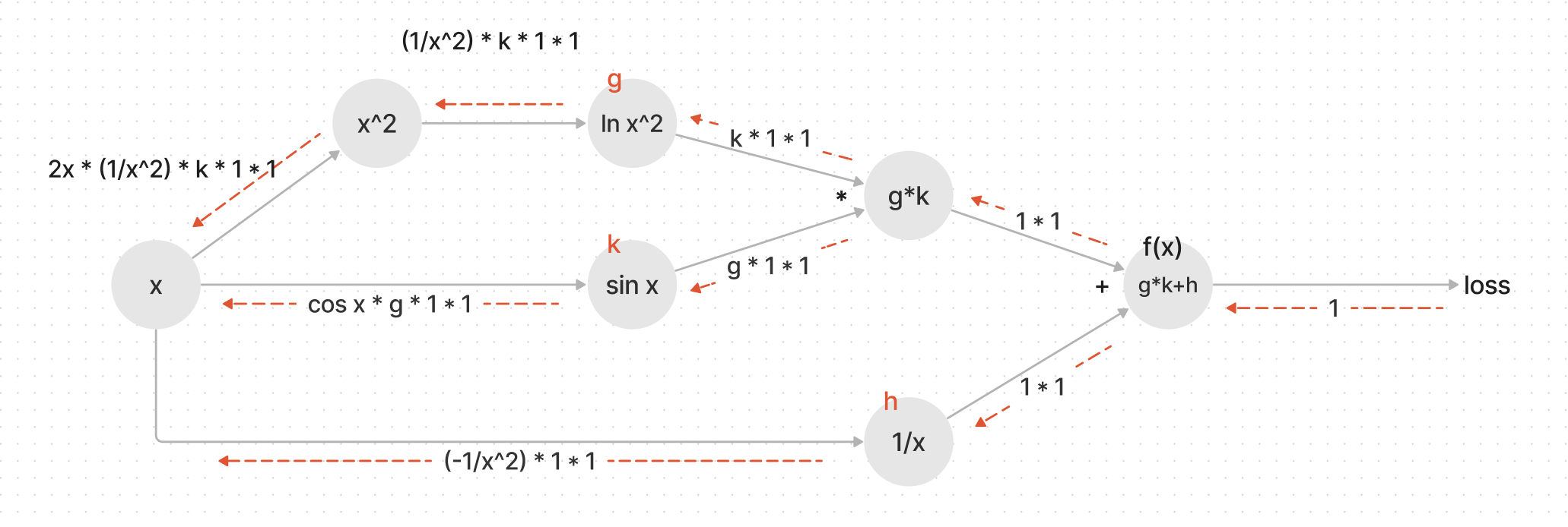
I have provided a diagram created using Mermaid that illustrates the detaching computation sections.
The solid lines represent the forward computation path, while the dashed lines indicate the backpropagation path.
I hope this helps you better understand the workflow of this functionality. Please let me know if there are any issues or corrections needed.