Auto Differentiation

I don’t quite understand 2.5.2.

My understanding is that by default the framework will convert the actual output matrix into a vector based on a “gradient vector” that we passed in. The description of this “gradient vector” is

which specifies the gradient of the differentiated function w.r.t self.

What does it mean? Does “gradient of differentiated function” mean “second order gradient”?

My answers to the questions: please point out if I am misunderstood anything

  1. Why is the second derivative much more expensive to compute than the first derivative?

Because instead of following the original computation graph, we need to construct a new one that corresponds to the calculation of first-order gradient?

  1. After running the function for backpropagation, immediately run it again and see what happens.

RuntimeError: Trying to backward through the graph a second time, but the saved intermediate results have already been freed. Specify retain_graph=True when calling backward the first time.

  1. In the control flow example where we calculate the derivative of d with respect to a , what would happen if we changed the variable a to a random vector or matrix. At this point, the result of the calculation f(a) is no longer a scalar. What happens to the result? How do we analyze this?

Directly changing would give the “blah blah … only scalar output” which is what 2.5.2 is talking about. I changed the code to

a = torch.randn(size=(3,), requires_grad=True)
d = f(a)
d.sum().backward()

and a.grad == d / a still gives true. This is because in the function, there is no cross-element operation. So each element of the vector is independent and doesn’t affect other element’s differentiation.

  1. Redesign an example of finding the gradient of the control flow. Run and analyze the result.

SKIP

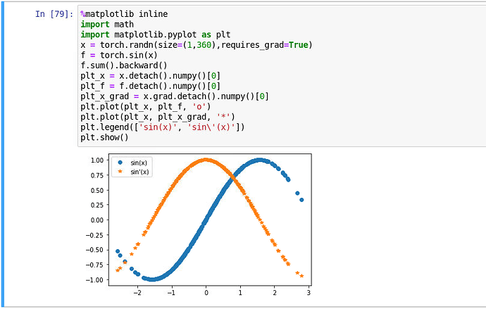
  1. Let $f(x) = \sin(x)$. Plot $f(x)$ and $\frac{df(x)}{dx}$, where the latter is computed without exploiting that $f’(x) = \cos(x)$.
import numpy as np
from d2l import torch as d2l
x = np.linspace(- np.pi,np.pi,100)
x = torch.tensor(x, requires_grad=True)
y = torch.sin(x)
y.sum().backward()

d2l.plot(x.detach(),(y.detach(),x.grad),legend = (('sin(x)',"grad w.s.t x")))
2 Likes

Hi @SONG_PAN, this is a first order gradient. The gradient is only available after we differentiate the function. :wink:

Hi, May I confirm my understanding about the auto differentiation of Python control flow?
I assume, as long as the Python control flow is established by functions and variables from Pytorch, then the auto differentiation is doable. Am I right on this? No other functions should be involved such as sin() from math package(have to use sin() from Pytorch instead if I want auto differentiation).


I tried. Did you mean this? @Aaron_L

I guess you can replace
for i in range(100):
y[i].backward(retain_graph = True)

with the following sentence:
y.sum().backward(retain_graph = True)

Anyone know how the backpropagation of CNN and RNN works? Are there any step by step tutorials to show the derivation? Thanks!

@gary

“Searching” is the best way to solve common questions like this.
Do you really want to learn? Or you only want to ask to act like a learner.
CNN: TODO:for you
RNN: http://preview.d2l.ai/d2l-en/master/chapter_recurrent-neural-networks/bptt.html

How about:
x = np.linspace(- np.pi,np.pi,100)
x = torch.tensor(x, requires_grad=True)
y = torch.sin(x)
z = y.sum()
z.backward()

d2l.plot(x.detach(),(y.detach(),x.grad),legend = (('sin(x)','grad w.s.t x')))

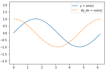
My solution to the last exercise

import torch
import matplotlib.pyplot as plt
import numpy as np
import math
%matplotlib inline

x = torch.arange(0, 2*math.pi, 0.1)
x.requires_grad_(True)
y = torch.sin(x).sum().backward() #Derivando y respecto a x

dy_dx = x.grad

x = x.detach().numpy()

y = np.sin(x)
dy_dx = dy_dx.numpy()

fig = plt.figure()
plt.plot(x, y, ‘-’, label = ‘y = sin(x)’)
plt.plot(x, dy_dx, ‘–’, label =’ dy_dx = cos(x)’)
plt.axis(‘equal’)
leg = plt.legend();

image

My solution to the last exercise

x = torch.arange(-np.pi, np.pi, 0.1, requires_grad=True)
y = torch.sin(x)
y.sum().backward()
x.grad

Exercise 1. The second derivative is much more expensive because, for a function f with n variables, the Hessian Matrix has elements while the gradient vector has n elements. In other words, there are possible second order derivatives ( ∂²f/∂x1², ∂²f/∂x1∂x2, …) while there are n possible first order derivatives (∂f/∂x1, ∂f/∂x2, …, ∂f/∂xn).

Backward for Non-Scalar Variables:

Seems, in the text, by calculating y.backward(torch.ones(len(x))), we contract the Jacobian over the 4 components of y(x). The Jacobian is a 4x4 matrix. I can extract each column via y.backward(torch.tensor([1,0,0,0])), #where i shift the 1 to each of the 4 column slots.
Is this best way to calculate the Jacobian?

My anwser for ex 2 3 4,welcom to tell me if you find any error

'''
ex.2
Aafter running the function for backpropagation, immediately run it again and see what hap-
pens. Why?

reference:
[https://blog.csdn.net/rothschild666/article/details/124170794](https://blog.csdn.net/rothschild666/article/details/124170794)
'''
import torch
x = torch.arange(4.0, requires_grad=True)
x.requires_grad_(True)
y = 2 * torch.dot(x, x)
y.backward(retain_graph=True)#need to set para = Ture
y.backward()
x.grad

out for ex2:
tensor([ 0., 8., 16., 24.])

'''
ex.3
In the control flow example where we calculate the derivative of d with respect to a, what
would happen if we changed the variable a to a random vector or a matrix? At this point, the
result of the calculation f(a) is no longer a scalar. What happens to the result? How do we
analyze this?


reference:
[https://www.jb51.net/article/211983.htm](https://www.jb51.net/article/211983.htm)
'''
import torch
def f(a):
    b = a * 2
    while b.norm() < 1000:
        b = b * 2
    if b.sum() > 0:
        c = b
    else:
        c = 100 * b
    return c
a = torch.randn(size=(2,3), requires_grad=True)
#a = torch.tensor([1.0,2.0], requires_grad=True)
print(a)
d = f(a)
d.backward(d.detach())#This is neccesary, I don't know why, is it because there are b and c in the function?
#d.backward()#wrong
print(a.grad)

out for ex3:
tensor([[-0.6848, 0.2447, 1.5633],
[-0.1291, 0.2607, 0.9181]], requires_grad=True)
tensor([[-179512.9062, 64147.3203, 409814.3750],
[ -33844.5430, 68346.7969, 240686.7344]])

'''
ex.4
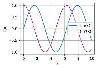
Let f (x) = sin(x). Plot the graph of f and of its derivative f ′ . Do not exploit the fact that
f ′ (x) = cos(x) but rather use automatic differentiation to get the result.
'''
#suppose the functions in 2.4.2Visualization Utilities has been constructed in d2l
from d2l import torch as d2l
x = d2l.arange(0,10,0.1, requires_grad = True)
y = d2l.sin(x)
y.backward(gradient=d2l.ones(len(y)))#y.sum().backward() can do the same thing
#.detach.numpy() is needed because x is set to requires_grad = True
d2l.plot(x.detach().numpy(), [y.detach().numpy(),x.grad], 'x', 'f(x)', legend = ['sin(x)','sin\'(x)'])

out for ex4:
图片

This link https://mblondel.org/teaching/autodiff-2020.pdf may help to answer the 8th question.

Answer for 4th question : Google Colab

Can someone please explain the result of 2.5.1 to me. I understand how the first function is just y = 2x^2, but creating the new function that is y = x.sum(), just returns 6. Is this conceptually 6x or is it just 6 or is this just x (i’m assuming the third because that’s the only way we can get 1 as the gradient all the time) or am i missing something?

My understanding about 2.5.1’s pytorch code blocks:

y = x.sum() is just a way of defining a computational graph in PyTorch, which means evaluating each component of x and adding them up. Gradients are computed on each component of x, NOT on the y graph. Evaluating gradient on a component of x means computing for y_i = x_i (which yields 1).

The same principal applies to the y = 2 * x^Tx part, y is NOT 2x^2, it’s a computational graph for evaluating 2 * x^Tx where each component of it is actually y_i = 2 * x_i * x_i. So the graph y is in fact sum { 2 * x_i * x_i }.

HTH

Can someone help with Questions 5 and 6. Is this a pen-paper question, writing down backprop for the computation graph, or is this supposed to be implemented (if yes, then can someone elaborate more on it or provide a solution.)

Also problems 7, 8 are difficult ones, but at least there is a good resource provided by Denis Kazakov.