My anwser for ex 2 3 4,welcom to tell me if you find any error
'''
ex.2
Aafter running the function for backpropagation, immediately run it again and see what hap-
pens. Why?

reference:
[https://blog.csdn.net/rothschild666/article/details/124170794](https://blog.csdn.net/rothschild666/article/details/124170794)
'''
import torch
x = torch.arange(4.0, requires_grad=True)
x.requires_grad_(True)
y = 2 * torch.dot(x, x)
y.backward(retain_graph=True)#need to set para = Ture
y.backward()
x.grad
out for ex2:
tensor([ 0., 8., 16., 24.])
'''
ex.3
In the control flow example where we calculate the derivative of d with respect to a, what
would happen if we changed the variable a to a random vector or a matrix? At this point, the
result of the calculation f(a) is no longer a scalar. What happens to the result? How do we
analyze this?


reference:
[https://www.jb51.net/article/211983.htm](https://www.jb51.net/article/211983.htm)
'''
import torch
def f(a):
    b = a * 2
    while b.norm() < 1000:
        b = b * 2
    if b.sum() > 0:
        c = b
    else:
        c = 100 * b
    return c
a = torch.randn(size=(2,3), requires_grad=True)
#a = torch.tensor([1.0,2.0], requires_grad=True)
print(a)
d = f(a)
d.backward(d.detach())#This is neccesary, I don't know why, is it because there are b and c in the function?
#d.backward()#wrong
print(a.grad)
out for ex3:
tensor([[-0.6848, 0.2447, 1.5633],
[-0.1291, 0.2607, 0.9181]], requires_grad=True)
tensor([[-179512.9062, 64147.3203, 409814.3750],
[ -33844.5430, 68346.7969, 240686.7344]])
'''
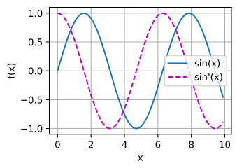
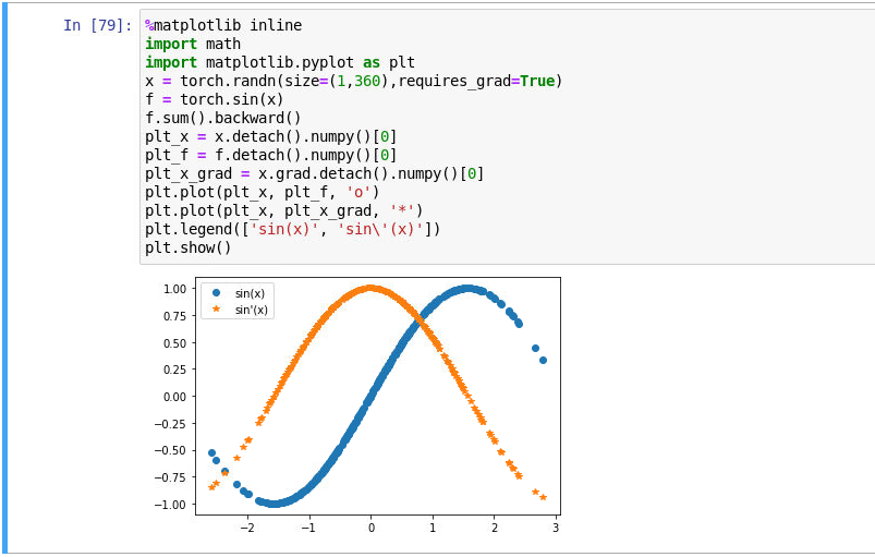
ex.4
Let f (x) = sin(x). Plot the graph of f and of its derivative f ′ . Do not exploit the fact that
f ′ (x) = cos(x) but rather use automatic differentiation to get the result.
'''
#suppose the functions in 2.4.2Visualization Utilities has been constructed in d2l
from d2l import torch as d2l
x = d2l.arange(0,10,0.1, requires_grad = True)
y = d2l.sin(x)
y.backward(gradient=d2l.ones(len(y)))#y.sum().backward() can do the same thing
#.detach.numpy() is needed because x is set to requires_grad = True
d2l.plot(x.detach().numpy(), [y.detach().numpy(),x.grad], 'x', 'f(x)', legend = ['sin(x)','sin\'(x)'])
out for ex4: