Whether we include a corresponding bias penalty b^2 can vary across implementations, and may vary across layers of a neural network. Often, we do not regularize the bias term of a network’s output layer.
Can you explain b^2 in detail?

Hi @StevenJokes, thanks for the feedback, we will fix it!
Hi @StevenJokes
4.5.1. Squared Norm Regularization
Whether we include a corresponding bias penalty b^2 can vary across implementations, and may vary across layers of a neural network. Often, we do not regularize the bias term of a network’s output layer. Can you explain b^2 in detail?
Great question! I hardly ever see $b^2$ Generally, applying weight decay to the bias units usually makes only a small difference to the final network.
1 reply
So it just means that bias penalty is not negative?
b is not same as the b in wx+b?

@goldpiggy
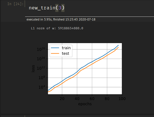
I tried to implement the code for train_concise on my own and my loss kept increasing exponentially instead of decreasing:
Here is my code:
def new_train(lambd):
net=nn.Sequential(nn.Linear(num_inputs,1))
for param in net.parameters():
    param.data.normal_()
loss=nn.MSELoss()
num_epochs=100
lr=0.03
trainer=torch.optim.SGD([{"params":net[0].weight,'weight_decay':lambd},
                         {"params":net[0].bias}],lr=lr)
animator = d2l.Animator(xlabel='epochs', ylabel='loss', yscale='log',
                        xlim=[1, num_epochs], legend=['train', 'test'])
for epoch in range(num_epochs):
    for X,y in train_iter:
        with torch.enable_grad():
            trainer.zero_grad()
            l=loss(net(X),y)
        l.backward()
        trainer.step()
    if epoch%5==0:
         animator.add(epoch, (d2l.evaluate_loss(net, train_iter, loss),
                             d2l.evaluate_loss(net, test_iter, loss)))
print('L1 norm of w:', net[0].weight.norm().item())
I compared my code to the code given in the book to find where I am going wrong but I can’t figure out where I made an error and what is causing this to happen.
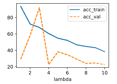
Intersestingly, if I increase the value of lambd to say 10, I get low generalization error but the train accuracy seems to be somewhat erratic:
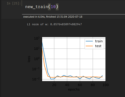
Any ideas on this as well?
1 reply
Hey @Kushagra_Chaturvedy, the learning rate is 0.003, while yours is different. Tuning learning rate is kind of tricky, not too small and not too high.
2 replies
Ok, I didn’t know that the learning rate could cause this much disparity in results. Thanks!
Is b in b^2 same as the b in wx+b?

I think the idea is that W is a really high-dimensional vector because there are so many weights. b is relatively low-dimensional, so regularizing b has a much smaller effect.
1 reply
Hello. I have two questions about this notebook. (1) Do I understand correctly that “weight decay” is a generic term for any regularization that involves adding some kind of norm of W (regardless of which norm) to the loss? (2) Is it not possible to add L1 regularization to the optim.SGD input? The docstring only lists L2 norm.
Thanks!
3 replies
Great question! Weight decay ideally should be mathematically equivalent to L2 Regularization. But be carefully when you implement it in code, this article indicates that different frameworks might be slightly different.
You are maybe right.
Does that mean we can use w and b as bias penalty at the same time or separately?
Hi @StevenJokes and @Steven_Hearnt, great questions! L1 regularization is applicable if you specify how to handle the in-differentiable case (x=0) .

Hi @StevenJokes, I might be late to the party but would like to take a stab at it from a theoretical point of view rather than practical (which has already been covered). If we regularize the bias term (b) by adding the penalty term b^2, the network would end up learning a very small value of bias term in the case where we constraint the model a lot (i.e. lambda is very big). In such a case, model would not have any average value and thus it would be predicting some value near to zero every time. So, in order to avoid such a scenario, maybe bias term isn’t regularized in the last layer.
1 reply
Why
“the network would end up learning a very small value of bias term”?
What does your “lambda” mean?
1 reply
Lambda is the constraint imposed on the L2 norm in the loss function. It is defined in 4.5.2. If we set lambda to a very large number and include bias term in the L2 norm as well, gradient descent will set bias term to an extremely small number as well. All of this is mentioned in the section 4.5
1 reply
…still can’t understand “the affine aspect”.
Some related papers? @kusur

In 4.5.1
The technique is motivated by the basic intuition that among all functions f, the function f=0 (assigning the value 0 to all inputs) is in some sense the simplest , and that we can measure the complexity of a function by its distance from zero.
Why is f = 0 considered the simplest? What does it mean for a function to be simple/complex in this context? Why is a function’s distance from zero, a measure of its complexity?
The most common method for ensuring a small weight vector is to add its norm as a penalty term to the problem of minimizing the loss
What does a weight vector being “small” mean? Like, number of elements in the weight vector (length of the weight vector)?
1 reply
Hi @tinkuge, great questions!
f = 0 means no regularization, that’s why it is the simplest (no computation here ![]() ). Check the Lp distance and it should give you better answer.
). Check the Lp distance and it should give you better answer.
“small” refers each weight element’s value is small, such as following within range [-1, 1].

Any idea on how do I implement an L1 regularized weight decay using
torch.optim.SGD
As per PyTorch documentation torch.optim — PyTorch 2.1 documentation it seems like the weight_decay parameter only implements L2 regularization.
2 replies
It looks like l1 norm has to be implemented using lower-level api
any one has idea about question 6? thx

Is there someone can share the idea about question 6? thx

It seem that a model with no regularization is better than a model with regularization in my case. Although the norm of the weights is significantly lower in the model with regularization, the plots are better in the unregularized one. Another problem is that the loss in my validation data is lower than the training loss. Here is my code:
import torch
from torch.utils.data import TensorDataset, DataLoader
import matplotlib.pyplot as plt

def synthetic_data(true_w, true_b, n):
    X = torch.normal(0, 0.01, (n, len(true_w)))
    y = torch.matmul(X, true_w) + true_b
    y += torch.normal(0, 0.001, y.shape)
    return X, y.reshape((-1, 1))

def load_array(array, batch_size, is_train=False):
    ''' Change array to a torch data iterator '''
    dataset = TensorDataset(*array)
    return DataLoader(dataset, batch_size=batch_size, shuffle=is_train)

n_train, n_test, n_inputs, batch_size = 20, 100, 200, 5

true_w = torch.ones((n_inputs, 1)) * 0.01
true_b = 0.05

train_data, train_labels = synthetic_data(true_w, true_b, n_train)
train_iter = load_array((train_data, train_labels), batch_size, is_train=True)
test_data, test_labels = synthetic_data(true_w, true_b, n_test)
test_iter = load_array((test_data, test_labels), batch_size)

# build the model
def linreg(X):
    return X@W + b

# initialize the weights
W = torch.normal(0, 1, (n_inputs, 1), requires_grad=True)
b = torch.zeros(1, requires_grad=True)

# define the loss function
def MSELoss(y_hat, y):
    return (y_hat - y) ** 2 / 2

# define the L2 regularization term
def L2_penality(W):
    return torch.norm(W) / 2

# Define the optimizer
def SGD(params, batch_size):
    with torch.no_grad():
        for param in params:
            param -= lr * param.grad / batch_size
            param.grad.zero_()

class Accumulator:
    def __init__(self, n):
        self.data = [0.0] * n

    def add(self, *args):
        self.data = [a + float(b) for a, b in zip(self.data, args)]

    def reset(self):
        self.data = [0.0] * len(self.data)

    def __getitem__(self, index):
        return self.data[index]

def evaluate(data_iter):
    metric = Accumulator(2)
    with torch.no_grad():
        for X, y in data_iter:
            l = MSELoss(linreg(X), y)
            metric.add(float(l.sum().item()), len(y))
    return metric[0] / metric[1]

# Write the training loop
epochs, lr = 100, 0.003
weight_decay = 0

train_loss = []
val_loss = []

train_metric = Accumulator(2)
for epoch in range(epochs):
    for X, y in train_iter:
        l = MSELoss(linreg(X), y) + weight_decay * L2_penality(W)
        l.sum().backward()
        SGD([W, b], batch_size)
        train_metric.add(float(l.sum().item()), len(y))

    train_loss.append(train_metric[0] / train_metric[1])
    train_metric.reset()

    # test the validation loss
    l = evaluate(test_iter)
    val_loss.append(l)

##    print("Epoch {}/{}   loss:  {:.5f}    val_loss:  {:.5f}".format(epoch+1, epochs, train_loss[-1], val_loss[-1]))
print("Weight Norm: ", torch.norm(W).item())


plt.plot(range(len(train_loss)), train_loss, label='Train loss')
plt.plot(range(len(val_loss)), val_loss, label='Validation loss')
plt.xlabel("Epochs")
plt.ylabel("Loss")
plt.title("Training and validation loss")
plt.legend()
plt.show()
First post!  Thanks for this amazing book.
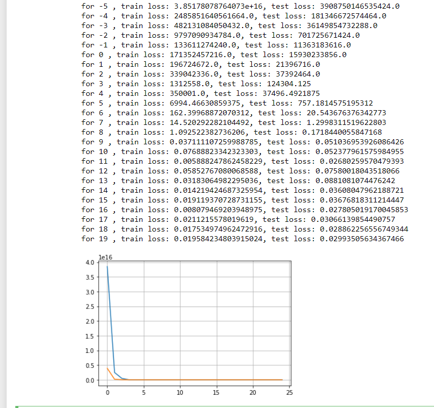
Also, I tried to plot train and test loss vs the choice of lambda. We can see that the training loss increases and test loss first decreases then stays mostly constant (see exact values below)
So, is the first value where test loss decreases before staying stagnant (i.e. lambda=1) is the best regularization parameter for this problem @goldpiggy can you suggest if this is a ok heuristic?

srno lambda train_loss test_loss
0 0 2.360348e-13 1.914223
1 1 3.561247e-04 0.035403
2 2 1.136713e-03 0.018138
3 3 2.143079e-03 0.017133
4 4 3.240126e-03 0.017512
5 5 4.373294e-03 0.017590
6 6 5.604185e-03 0.017622
7 7 6.343381e-03 0.017295
8 8 7.639927e-03 0.017984
9 9 8.753147e-03 0.017798
10 10 9.767077e-03 0.017654

#https://stackoverflow.com/questions/42704283/adding-l1-l2-regularization-in-pytorch
def l1_norm_with_abs(w):
return torch.abs(w).sum()test accuracy as a function of λ. What do you observe?
matter?
2 we used ∑
i
|wi
| as our penalty
of choice (L1 regularization)?
# training for l1 norm

model = nn.Sequential(nn.Linear(num_inputs, 1))

for param in model.parameters():

    param.data.normal_()

    print(l1_norm(param.detach()))


loss = nn.MSELoss()

optimizer = torch.optim.SGD(model.parameters(), lr = 0.03)

valid_loss_array = []

for epoch in range(20):

    current_loss = 0

    current_number = 0

    for X, y in valid_dataloader:

        l = loss(model(X),y) - l1_norm_with_abs(model[0].weight)


        optimizer.zero_grad()

        l.backward()

        optimizer.step()


        current_loss += l.detach()

        current_number += len(y)


    valid_loss_array.append(current_loss/current_number)

plt.plot(range(20), valid_loss_array)

plt.grid(True)

plt.show()
(cant upload the graph here only onw pic per post)
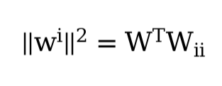
2 = w⊤w. Can you find a similar equation for matrices (see the Frobenius
norm in Section 2.3.10)?
weight decay, increased training, and the use of a model of suitable complexity, what other
ways can you think of to deal with overfitting?
P(w | x) ∝ P(x | w)P(w). How can you identify P(w) with regularization?
hi can how are you getting this graph? mine is at loggerheads with yours


Even I have no clue about this question.
HI I still didntget it, I am really challenged at maths I think! XD Hey but are you following the book ? I was lookingfor peoplegoing through this book !
1 reply
Yes, I am going through the book. Currently in chapter 5.
For this problem you can look at trace of the matrix.
For this, I think that this will involve proving it through log-likelihood method. if we assume P(w) to be normal distribution with mean 0 and variance = sigma^2, we might be able to derive the L2 regularization using Max Likelihood

I would love some insight into problem 6! I can’t make any headway. Loving the book so far. Thanks

I think this post does a good job at discussing Q6

Here are my opinions about the exs.
ex.1
I close the lot in d2l.Module.
@d2l.add_to_class(d2l.Module)
def training_step(self, batch):
    l = self.loss(self(*batch[:-1]), batch[-1])
    #self.plot('loss', l, train=True)
    return l
@d2l.add_to_class(d2l.Module)
def validation_step(self, batch):
    l = self.loss(self(*batch[:-1]), batch[-1])
    #self.plot('loss', l, train=False)
    return l
Then I use this code snippet to test lambda from 1 to 10
import numpy as np

data = Data(num_train=100, num_val=100, num_inputs=200, batch_size=20)
trainer = d2l.Trainer(max_epochs=10)
test_lambds=np.arange(1,11,1)
board = d2l.ProgressBoard('lambda')

def accuracy(y_hat, y):
    return (1 - ((y_hat - y).mean() / y.mean()).abs()) * 100

def train_ex1(lambd):
    model = WeightDecay(wd=lambd, lr=0.01)
    model.board.yscale='log'
    trainer.fit(model, data)
    y_hat = model.forward(data.X)
    acc_train = accuracy(y_hat[:data.num_train], data.y[:data.num_train])
    acc_val = accuracy(y_hat[data.num_train:], data.y[data.num_train:])
    return acc_train, acc_val

for item in test_lambds:
    acc_train, acc_val = train_ex1(item)
    board.draw(item, acc_train.to(d2l.cpu()).detach().numpy(), 'acc_train', every_n=1)
    board.draw(item, acc_val.to(d2l.cpu()).detach().numpy(), 'acc_val', every_n=1)
The output of accuracy of different lambda goes like this:
ex.2
I think there may be an analytical solution of lambda if the weights w have already been set after training, and the validation set is fixed, but this procedure gives no credit to any different validation set, so this kind of optimal makes no sense.
I think it doesn’t matter if the lambda is optimal, cause in practice, I can test a set of options and choose one that is good enough to be my lambda.
ex.3
ex.6
Regularization adds some limit on the parameters of a model before the training, that is somehow like a prior in Bayesian estimation.

what is a scratch? please define scratch.

My solutions to the exs: 3.7

I’m seeing a similar L2 norm of the weights between the example without regularization and the example using ‘weight_decay’ in torch.optim.SGD.
The examples in the book show this as well, whereas the L2 norm of the weights is 10 times smaller for the WeightDecayScratch using a lambda of 3.
Why might we expect this?

I am trying to implement weight decay from scratch, however no matter what I set lambda to, I notice the validation loss is always constant. Is there something wrong with my code?
class Data():
def init(self, num_train, num_val, num_inputs, batch_size):
self.batch_size = batch_size
n = num_train + num_val
self.X = torch.randn(n, num_inputs)
noise = torch.randn(n, 1) * .01
w, b = torch.ones((num_inputs, 1)) * .01, .05
self.y = torch.matmul(self.X, w) + b + noise
self.num_train = num_traindef get_trainloader(self): tensorData = TensorDataset(self.X[:self.num_train], self.y[:self.num_train]) return DataLoader(tensorData, batch_size=self.batch_size, shuffle=True) def get_testloader(self): tensorData = TensorDataset(self.X[self.num_train:], self.y[self.num_train:]) return DataLoader(tensorData, batch_size = self.batch_size, shuffle = False)class WeightDecay():
def init(self, num_inputs, lambd, lr):
self.num_inputs = num_inputs
self.lambd = lambd
self.lr = lr
self.net = nn.LazyLinear(1)
self.net.weight.data.normal_(0, .01)
self.net.bias.data.fill_(0)def forward(self, x): return self.net(x) def loss(self, yhat, y): loss_fun = nn.MSELoss()(yhat, y) L2_reg = self.lambd * ((self.net.weight ** 2).sum() / 2) return loss_fun + L2_reg def configure_optimizer(self): return torch.optim.SGD(self.net.parameters(), self.lr, weight_decay=0)data = Data(num_train=20, num_val=100, num_inputs=200, batch_size=5)
model = WeightDecay(200, lambd=0.1, lr=0.01)
optim = model.configure_optimizer()
train_data = data.get_trainloader()
test_data = data.get_testloader()for i in range(10):
train_loss = 0
for X, y in train_data:
preds = model.forward(X)
lossfun = model.loss(preds, y)
train_loss += lossfun
optim.zero_grad()
lossfun.backward()
optim.step()with torch.no_grad(): test_loss = 0 for X, y in test_data: preds = model.forward(X) lossfun = model.loss(preds, y) test_loss += lossfun print(f"Avg loss for epoch {i + 1} on train is {train_loss / len(train_data)}") print(f"Avg loss for epoch {i + 1} on test is {test_loss / len(test_data)}")
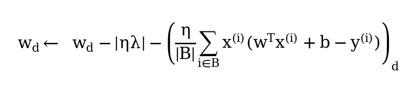
\lambda, the validation loss goes down far more quickly in early epochs. But no matter how large my setting of \lambda, the validation loss doesn’t seem to go far below 10e-2. For extremely large values, the model fails to converge at all.\lambda well into the range of 10-50! But in practice, I’m not sure you’d want to use a value so extreme - this example is somewhat contrived, and exaggerates the effect of weight decay. Using values this large in practice would hurt the model’s capacity.\|\mathbf w\|^2, our update to each parameter w_i is equivalent to \eta \lambda \cdot \mathbf w_i. If we used |\mathbf w|, our updates would not scale relative to the weights, and would be a constant \eta \lambda times the sign of w.\| A \|_F^2 = \text{trace}(A^T A). Intuitively, the diagonal entries on the gram matrix of A are where the dot product of each column with itself is located - these are the sums of the squares of each column. When we add them up, all entries are included.
Apart from data augmentation, regularization, and choosing a model with suitable complexity, for deep learning methods, we can consider using dropout (to avoid co-adaption of features), early stopping, and parameter sharing (to reduce the number of parameters, such as in CNN). For tree-based methods, we can consider ensemble models. For example, a single decision tree is prone to overfitting, but by creating a random forest, we can reduce variance and counter overfitting.
L1 regularization corresponds to a Laplace prior, while L2 regularization corresponds to a Gaussian prior.