It looks like l1 norm has to be implemented using lower-level api
any one has idea about question 6? thx
Is there someone can share the idea about question 6? thx
It seem that a model with no regularization is better than a model with regularization in my case. Although the norm of the weights is significantly lower in the model with regularization, the plots are better in the unregularized one. Another problem is that the loss in my validation data is lower than the training loss. Here is my code:
import torch
from torch.utils.data import TensorDataset, DataLoader
import matplotlib.pyplot as plt

def synthetic_data(true_w, true_b, n):
    X = torch.normal(0, 0.01, (n, len(true_w)))
    y = torch.matmul(X, true_w) + true_b
    y += torch.normal(0, 0.001, y.shape)
    return X, y.reshape((-1, 1))

def load_array(array, batch_size, is_train=False):
    ''' Change array to a torch data iterator '''
    dataset = TensorDataset(*array)
    return DataLoader(dataset, batch_size=batch_size, shuffle=is_train)

n_train, n_test, n_inputs, batch_size = 20, 100, 200, 5

true_w = torch.ones((n_inputs, 1)) * 0.01
true_b = 0.05

train_data, train_labels = synthetic_data(true_w, true_b, n_train)
train_iter = load_array((train_data, train_labels), batch_size, is_train=True)
test_data, test_labels = synthetic_data(true_w, true_b, n_test)
test_iter = load_array((test_data, test_labels), batch_size)

# build the model
def linreg(X):
    return X@W + b

# initialize the weights
W = torch.normal(0, 1, (n_inputs, 1), requires_grad=True)
b = torch.zeros(1, requires_grad=True)

# define the loss function
def MSELoss(y_hat, y):
    return (y_hat - y) ** 2 / 2

# define the L2 regularization term
def L2_penality(W):
    return torch.norm(W) / 2

# Define the optimizer
def SGD(params, batch_size):
    with torch.no_grad():
        for param in params:
            param -= lr * param.grad / batch_size
            param.grad.zero_()

class Accumulator:
    def __init__(self, n):
        self.data = [0.0] * n

    def add(self, *args):
        self.data = [a + float(b) for a, b in zip(self.data, args)]

    def reset(self):
        self.data = [0.0] * len(self.data)

    def __getitem__(self, index):
        return self.data[index]

def evaluate(data_iter):
    metric = Accumulator(2)
    with torch.no_grad():
        for X, y in data_iter:
            l = MSELoss(linreg(X), y)
            metric.add(float(l.sum().item()), len(y))
    return metric[0] / metric[1]

# Write the training loop
epochs, lr = 100, 0.003
weight_decay = 0

train_loss = []
val_loss = []

train_metric = Accumulator(2)
for epoch in range(epochs):
    for X, y in train_iter:
        l = MSELoss(linreg(X), y) + weight_decay * L2_penality(W)
        l.sum().backward()
        SGD([W, b], batch_size)
        train_metric.add(float(l.sum().item()), len(y))

    train_loss.append(train_metric[0] / train_metric[1])
    train_metric.reset()

    # test the validation loss
    l = evaluate(test_iter)
    val_loss.append(l)

##    print("Epoch {}/{}   loss:  {:.5f}    val_loss:  {:.5f}".format(epoch+1, epochs, train_loss[-1], val_loss[-1]))
print("Weight Norm: ", torch.norm(W).item())


plt.plot(range(len(train_loss)), train_loss, label='Train loss')
plt.plot(range(len(val_loss)), val_loss, label='Validation loss')
plt.xlabel("Epochs")
plt.ylabel("Loss")
plt.title("Training and validation loss")
plt.legend()
plt.show()First post!  Thanks for this amazing book.
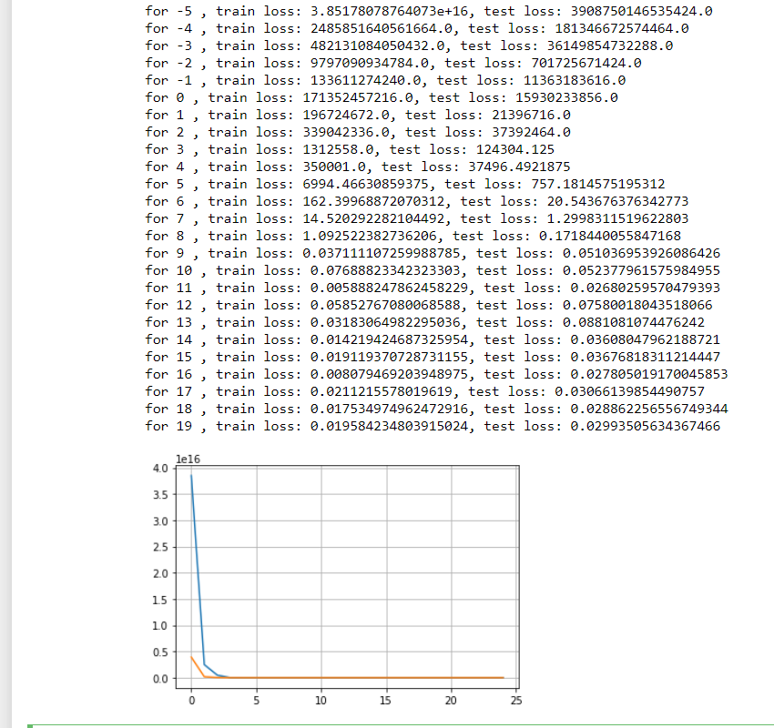
Also, I tried to plot train and test loss vs the choice of lambda. We can see that the training loss increases and test loss first decreases then stays mostly constant (see exact values below)
So, is the first value where test loss decreases before staying stagnant (i.e. lambda=1) is the best regularization parameter for this problem @goldpiggy can you suggest if this is a ok heuristic?

srno lambda train_loss test_loss
0 0 2.360348e-13 1.914223
1 1 3.561247e-04 0.035403
2 2 1.136713e-03 0.018138
3 3 2.143079e-03 0.017133
4 4 3.240126e-03 0.017512
5 5 4.373294e-03 0.017590
6 6 5.604185e-03 0.017622
7 7 6.343381e-03 0.017295
8 8 7.639927e-03 0.017984
9 9 8.753147e-03 0.017798
10 10 9.767077e-03 0.017654
#https://stackoverflow.com/questions/42704283/adding-l1-l2-regularization-in-pytorch
def l1_norm_with_abs(w):
return torch.abs(w).sum()Exercises and my answers
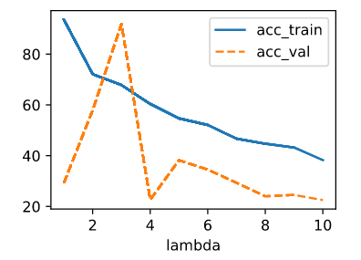
- Experiment with the value of λ in the estimation problem in this section. Plot training and
test accuracy as a function of λ. What do you observe?
- as we increase wd it is making better train and test loss graph
- Use a validation set to find the optimal value of λ. Is it really the optimal value? Does this
matter?
- the minimum loss is 0.02 at wd = 21-5 = 16. It is th eoptimal value for the validation set.
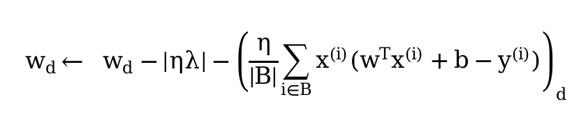
- What would the update equations look like if instead of ∥w∥
2 we used ∑
i
|wi
| as our penalty
of choice (L1 regularization)?
- It is strangely coming as linear
# training for l1 norm

model = nn.Sequential(nn.Linear(num_inputs, 1))

for param in model.parameters():

    param.data.normal_()

    print(l1_norm(param.detach()))


loss = nn.MSELoss()

optimizer = torch.optim.SGD(model.parameters(), lr = 0.03)

valid_loss_array = []

for epoch in range(20):

    current_loss = 0

    current_number = 0

    for X, y in valid_dataloader:

        l = loss(model(X),y) - l1_norm_with_abs(model[0].weight)


        optimizer.zero_grad()

        l.backward()

        optimizer.step()


        current_loss += l.detach()

        current_number += len(y)


    valid_loss_array.append(current_loss/current_number)

plt.plot(range(20), valid_loss_array)

plt.grid(True)

plt.show()
(cant upload the graph here only onw pic per post)
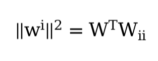
- We know that ∥w∥
2 = w⊤w. Can you find a similar equation for matrices (see the Frobenius
norm in Section 2.3.10)?
- This is Frobenius norm: f(αx) = |α|f(x). I dont understand.
- Review the relationship between training error and generalization error. In addition to
weight decay, increased training, and the use of a model of suitable complexity, what other
ways can you think of to deal with overfitting?
- larger data size, dropouts
- In Bayesian statistics we use the product of prior and likelihood to arrive at a posterior via
P(w | x) ∝ P(x | w)P(w). How can you identify P(w) with regularization?
- you ask good question but me no understand. how to get to p of w.
hi can how are you getting this graph? mine is at loggerheads with yours
- In Bayesian statistics we use the product of prior and likelihood to arrive at a posterior via 𝑃(𝑤∣𝑥)∝𝑃(𝑥∣𝑤)𝑃(𝑤). How can you identify 𝑃(𝑤) with regularization?
@goldpiggy Hi, 𝑃(𝑤∣𝑥)P(x) = 𝑃(𝑥∣𝑤)𝑃(𝑤). Here, P(w|x), P(x), P(w) can be acquired through statistics, so, P(w) can be found if we assume a linear model between P(w|x) *P(x) and p(x|w).
Is it correct?
Even I have no clue about this question.
I guess 4th will be trace(X’X) where X’ = X transpose
1 Like
HI I still didntget it, I am really challenged at maths I think! XD Hey but are you following the book ? I was lookingfor peoplegoing through this book !
Yes, I am going through the book. Currently in chapter 5.
For this problem you can look at trace of the matrix.
1 Like
For this, I think that this will involve proving it through log-likelihood method. if we assume P(w) to be normal distribution with mean 0 and variance = sigma^2, we might be able to derive the L2 regularization using Max Likelihood
I would love some insight into problem 6! I can’t make any headway. Loving the book so far. Thanks
I think this post does a good job at discussing Q6
Here are my opinions about the exs.
ex.1
I close the lot in d2l.Module.
@d2l.add_to_class(d2l.Module)
def training_step(self, batch):
    l = self.loss(self(*batch[:-1]), batch[-1])
    #self.plot('loss', l, train=True)
    return l
@d2l.add_to_class(d2l.Module)
def validation_step(self, batch):
    l = self.loss(self(*batch[:-1]), batch[-1])
    #self.plot('loss', l, train=False)
    return l
Then I use this code snippet to test lambda from 1 to 10
import numpy as np

data = Data(num_train=100, num_val=100, num_inputs=200, batch_size=20)
trainer = d2l.Trainer(max_epochs=10)
test_lambds=np.arange(1,11,1)
board = d2l.ProgressBoard('lambda')

def accuracy(y_hat, y):
    return (1 - ((y_hat - y).mean() / y.mean()).abs()) * 100

def train_ex1(lambd):
    model = WeightDecay(wd=lambd, lr=0.01)
    model.board.yscale='log'
    trainer.fit(model, data)
    y_hat = model.forward(data.X)
    acc_train = accuracy(y_hat[:data.num_train], data.y[:data.num_train])
    acc_val = accuracy(y_hat[data.num_train:], data.y[data.num_train:])
    return acc_train, acc_val

for item in test_lambds:
    acc_train, acc_val = train_ex1(item)
    board.draw(item, acc_train.to(d2l.cpu()).detach().numpy(), 'acc_train', every_n=1)
    board.draw(item, acc_val.to(d2l.cpu()).detach().numpy(), 'acc_val', every_n=1)
The output of accuracy of different lambda goes like this:
ex.2
I think there may be an analytical solution of lambda if the weights w have already been set after training, and the validation set is fixed, but this procedure gives no credit to any different validation set, so this kind of optimal makes no sense.
I think it doesn’t matter if the lambda is optimal, cause in practice, I can test a set of options and choose one that is good enough to be my lambda.
ex.3
ex.4
ex.5
I think if I can’t narrow gap between training error and generalizing error, there is also a great chance to reach overfitting, so I may use cross validation to make more use on the data I have now.
ex.6
Regularization adds some limit on the parameters of a model before the training, that is somehow like a prior in Bayesian estimation.
1 Like
what is a scratch? please define scratch.
I’m seeing a similar L2 norm of the weights between the example without regularization and the example using ‘weight_decay’ in torch.optim.SGD.
The examples in the book show this as well, whereas the L2 norm of the weights is 10 times smaller for the WeightDecayScratch using a lambda of 3.
Why might we expect this?