@goldpiggy
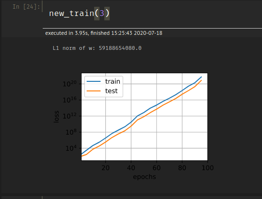
I tried to implement the code for train_concise on my own and my loss kept increasing exponentially instead of decreasing:
Here is my code:
def new_train(lambd):
net=nn.Sequential(nn.Linear(num_inputs,1))
for param in net.parameters():
    param.data.normal_()
loss=nn.MSELoss()
num_epochs=100
lr=0.03
trainer=torch.optim.SGD([{"params":net[0].weight,'weight_decay':lambd},
                         {"params":net[0].bias}],lr=lr)
animator = d2l.Animator(xlabel='epochs', ylabel='loss', yscale='log',
                        xlim=[1, num_epochs], legend=['train', 'test'])
for epoch in range(num_epochs):
    for X,y in train_iter:
        with torch.enable_grad():
            trainer.zero_grad()
            l=loss(net(X),y)
        l.backward()
        trainer.step()
    if epoch%5==0:
         animator.add(epoch, (d2l.evaluate_loss(net, train_iter, loss),
                             d2l.evaluate_loss(net, test_iter, loss)))
print('L1 norm of w:', net[0].weight.norm().item())
I compared my code to the code given in the book to find where I am going wrong but I can’t figure out where I made an error and what is causing this to happen.
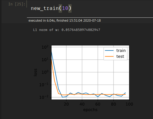
Intersestingly, if I increase the value of lambd to say 10, I get low generalization error but the train accuracy seems to be somewhat erratic:
Hey @Kushagra_Chaturvedy, the learning rate is 0.003, while yours is different. Tuning learning rate is kind of tricky, not too small and not too high.
I think the idea is that W is a really high-dimensional vector because there are so many weights. b is relatively low-dimensional, so regularizing b has a much smaller effect.
Hello. I have two questions about this notebook. (1) Do I understand correctly that “weight decay” is a generic term for any regularization that involves adding some kind of norm of W (regardless of which norm) to the loss? (2) Is it not possible to add L1 regularization to the optim.SGD input? The docstring only lists L2 norm.
Great question! Weight decay ideally should be mathematically equivalent to L2 Regularization. But be carefully when you implement it in code, this article indicates that different frameworks might be slightly different.
Hi @StevenJokes, I might be late to the party but would like to take a stab at it from a theoretical point of view rather than practical (which has already been covered). If we regularize the bias term (b) by adding the penalty term b^2, the network would end up learning a very small value of bias term in the case where we constraint the model a lot (i.e. lambda is very big). In such a case, model would not have any average value and thus it would be predicting some value near to zero every time. So, in order to avoid such a scenario, maybe bias term isn’t regularized in the last layer.
Lambda is the constraint imposed on the L2 norm in the loss function. It is defined in 4.5.2. If we set lambda to a very large number and include bias term in the L2 norm as well, gradient descent will set bias term to an extremely small number as well. All of this is mentioned in the section 4.5
Yep, If you include bias term in the l2_penalty, you set this parameter to a huge value, and train the model, you will notice that bias itself becomes very small. This removes the affine aspect of the transformation in the neural network
The technique is motivated by the basic intuition that among all functions f, the function f=0 (assigning the value 0 to all inputs) is in some sense the simplest , and that we can measure the complexity of a function by its distance from zero.
Why is f = 0 considered the simplest? What does it mean for a function to be simple/complex in this context? Why is a function’s distance from zero, a measure of its complexity?
The most common method for ensuring a small weight vector is to add its norm as a penalty term to the problem of minimizing the loss
What does a weight vector being “small” mean? Like, number of elements in the weight vector (length of the weight vector)?