I dont quite understand what Question 3 wants us to answer. When I change the original a to a random vector or matrix, nothing strange happens. Can anyone help me? What is the situation supposed to be?
- Because it has to invoke ‘backward()’ twice which definitely consumes more resources.
- RuntimeError occurs:
RuntimeError: Trying to backward through the graph a second time (or directly access saved tensors after they have already been freed). Saved intermediate values of the graph are freed when you call .backward() or autograd.grad(). Specify retain_graph=True if you need to backward through the graph a second time or if you need to access saved tensors after calling backward.
- RuntimeError occurs:
RuntimeError: grad can be implicitly created only for scalar outputs
def f(x):
    if torch.min(x) < 0:
        y = x * x
    else:
        y = torch.mean(x)
    return y
x = torch.randn(1, 5, requires_grad=True)
print(x)
y = f(x)
if y.dim() > 0:
    y = y.sum()
y.backward()
print(x.grad)
print(x.grad==2*x if torch.min(x)<0 else x.grad==1/x.shape[1]*torch.ones_like(x))
%run calculus.ipynb
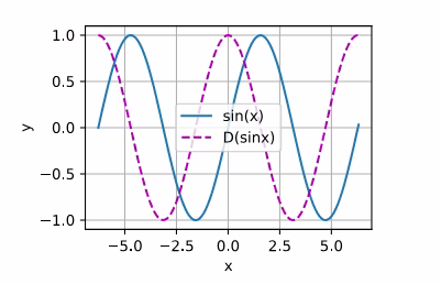
x = torch.arange(-2*torch.pi,2*torch.pi+0.1,0.1).requires_grad_()
f = lambda x: torch.sin(x)
f(x).sum().backward()
plot(x.detach(), [f(x).detach(), x.grad], 'x', 'y', legend=["sin(x)","D(sinx)"])
交作业:
- 为什么计算二阶导数比一阶导数的开销要更大?
我认为计算二阶导数需要更多的内存和计算资源。
内存:计算二阶导数时,需要存储更多的中间结果和梯度信息。
计算资源:计算二阶导数时,需要进行更多的计算操作,这增加了计算时间和资源消耗。
- 在运行反向传播函数之后,立即再次运行它,看看会发生什么。
发生了错误,因为在第一次backward()之后,梯度已经被清空了,所以在第二次backward()时,梯度为None
但我们可以通过设置retain_graph=True来保留计算图,这样就可以多次调用backward()了
# 课程的例1
import torch
x = torch.arange(4.0, requires_grad=True)
y = x * x # y 是矢量
y.sum().backward(retain_graph=True) # 由于 backward() 函数只能对标量调用,所以需要用 sum() 函数将 y 转换为标量
print(x.grad)
y.sum().backward()
print(x.grad)
- 在控制流的例子中,我们计算
d关于a的导数,如果将变量a更改为随机向量或矩阵,会发生什么?
def f(a):
b = a * 2
while b.norm() < 1000:
b = b * 2
if b.sum() > 0:
c = b
else:
c = 100 * b
return c
a = torch.randn(size=(7,), requires_grad=True) # a 现在是向量
d = f(a)
d.sum().backward()
print(a)
print(a.grad)
发生对应的长度变化。
梯度的本质是偏导数,而 PyTorch 会根据自动微分机制对每个分量求导。因此,
a 的梯度结构总是和 a 的结构一致:
标量:梯度是标量。ex: size=()
向量:梯度是每个分量的偏导数,形成向量。ex: size=(7,)
矩阵:梯度是每个分量的偏导数,形成矩阵。ex: size=(7,12)
- 重新设计一个求控制流梯度的例子,运行并分析结果。
def f(a):
if a > 0:
b = a * 2
else:
b = a * 3
while b.norm() < 1000:
b = b * 2
if b.sum() > 0:
c = b
else:
c = 100 * b
return c
# 创建一个随机标量 a,并设置 requires_grad=True
a = torch.randn(size=(), requires_grad=True)
# 计算 d = f(a)
d = f(a)
# 进行反向传播,计算梯度
d.sum().backward()
# 打印 a 的梯度
print("a 的值:", a)
print("a 的梯度:", a.grad)
运行结果:
a 的值: tensor(1.0775, requires_grad=True)
a 的梯度: tensor(1024.)
1 a 是一个随机标量,值为 1.0775
2 因为 a > 0,所以 b = a * 2,即 b = 1.0775 * 2 = 2.155。
进入 while 循环,不断将 b 乘以 2,直到 b.norm() 大于或等于 1000。
3 因为 b.sum() > 0,所以 c = b
4 d = c = b = 1103.36
进行反向传播,计算 a 的梯度。
因为 b 是通过不断乘以 2 得到的,所以 b 相对于 a 的梯度是 2^p,其中 p 是循环的次数。
在这个例子中,循环执行了 9 次,所以 p = 9,梯度是 2^9 = 512。
但是因为初始时 b = a * 2,所以总的梯度是 2 * 2^9 = 2^10 = 1024。
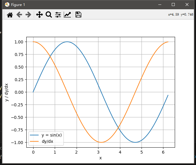
- 使f(x)=sin(x),绘制f(x)和df(x)/dx的图像,其中后者不使用f′(x)=cos(x)。
from math import pi
import matplotlib.pyplot as plt
def f(x):
y = torch.sin(x)
return y
x = torch.arange(0, 2*pi, 2*pi/100, requires_grad=True)
y = f(x)
y.sum().backward()
# 将张量从计算图中分离出来,然后转换为 numpy 数组并绘制 y = sin(x) 和 dy/dx 的图形
plt.plot(x.detach().numpy(), y.detach().numpy(), label='y = sin(x)')
plt.plot(x.detach().numpy(), x.grad.detach().numpy(), label='dy/dx')
# 添加标签和图例
plt.xlabel('x')
plt.ylabel('y / dy/dx')
plt.legend()
plt.grid(True)
plt.show()
踩了两个坑,关于只能对标量使用反向传播
1、这里的x和f(x)=sinx都是一个张量,画图的时候要用detach()方法看成标量,再进行画图。
d2l.plot(x.detach(), [f(x).detach(), x.grad], 'x', 'f(x)', figsize=(10, 2.5))
2、先对sinx求和得到张量,就可以得到x的梯度了。
f(x).sum().backward()
课后习题
- 为什么计算二阶导数比一阶导数的开销要更大?
答:因为二阶导数基于一阶导数 - 在运行反向传播函数之后,立即再次运行它,看看会发生什么。
答:RuntimeError: Trying to backward through the graph a second time (or directly access saved tensors after they have already been freed). Saved intermediate values of the graph are freed when you call .backward() or autograd.grad(). Specify retain_graph=True if you need to backward through the graph a second time or if you need to access saved tensors after calling backward. - 在控制流的例子中,我们计算
d关于a的导数,如果将变量a更改为随机向量或矩阵,会发生什么?
答:
def f(a):
    b = a * 2
    while b.norm() < 1000:
        b *= 2
    if b.sum() > 0:
        c = b
    else:
        c = 100 * b
    return c
f(x)返回的结果实际上一定是k*x,且是2的次方倍数
因此对x求导得到的就是k,也就是f(x) / x
a = torch.randn((2), requires_grad=True)
d = f(a)
d.sum().backward()
print(a.grad)
tensor([1024., 1024.])
正常输出,但是需要改成.sum()
- 重新设计一个求控制流梯度的例子,运行并分析结果。
答:
import math
def h(x):
    for i in range(3):
        x = torch.exp(x)
    return x

i = torch.randn((1), requires_grad=True)
j = h(i)
j.backward()
print(i.grad)
tensor([2.0552e+08]),梯度有点小炸但是没关系。
如果是非标量可以采用.mean()函数进行计算
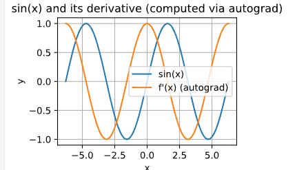
- 使 f(x)=sin(x) ,绘制f(x)和df(x)/dx的图像,其中后者不使用f’(x)=cos(x)。
答:
我也是啊,朋友你解决了这个问题了吗,一用d2l.plot就挂掉了
一开始q确实是叶子张量,但在进行reshape操作之后,q不再是叶子张量。因为reshape操作会创建一个新的张量,尽管他们的restorage(内存区域)一样。你应该使用中间变量去接收reshape后的张量
我这样理解的😂
要把张量转化为numpy,y.detach().numpy()
import torch
import d2l
x = torch.arange(-10, 10, 0.05, requires_grad=True)
y = torch.sin(x)
y.backward(torch.ones_like(y))
y_d = x.grad
d2l.torch.plot(x.detach(), [y.detach(), y_d],
‘x’, ‘f(x)’, legend=[‘f(x)=sin(x)’, “f’(x)=cos(x)”],figsize=[5,5])
第二问,出现报错Trying to backward through the graph a second time, but the saved intermediate results have already been freed. Specify retain_graph=True when calling .backward() or autograd.grad() the first time.
第一句话说的是:试图第二次反向传播计算图,但保存的中间结果已经被释放。
这是因为在默认情况下,Pytorch为了节省内存,会在每次.backward( )之后释放计算图,而计算图包含了反向传播所需的中间结果。
第二句话提供了解决办法:在第一次调用 .backward() 或 autograd.grad() 时指定retain_graph=True。
指定retain_graph=True也就是保留计算图,使其后续可以继续被使用。其中的一个应用是高阶导数计算,由于需要多次求导,或者说多次运行反向传播函数,因此需要保留计算图。
由于保留计算图会占用内存,因此计算高阶导数比计算低阶导数的开销要更大,这也回应了第一问。
第三问,在Pytorch中只有输出为标量时可以隐式创建梯度。对于标量函数,梯度明确定义为一个向量,而对于非标量函数,导数为雅克比矩阵。对非标量张量调用 .backward(),PyTorch会将其转换为标量处理,但需要指定如何将非标量张量转化为标量,即指定梯度权重。
可以通过以下方式显式指定梯度权重:
y.sum().backward():对雅克比矩阵中的每一个元素分配权重1,然后进行求和降维(y1, y2, …,yn对x1的梯度求和,得到x1关于损失的梯度)
y.mean().backward():对雅克比矩阵中的每一个元素分配权重1/n(n为y中的元素),然后进行求和降维(y1, y2, …,yn对x1的梯度都乘上1/n再求和,得到x1关于损失的梯度)
y.backward(gradient_weights) :对雅可比矩阵中的每一个元素分配特定的权重(y1, y2, …,yn对x1的梯度都分别乘上设定好的权重再求和,得到x1关于损失的梯度)
目前教材里的例子输入元素和输出元素之间似乎都是一一对应关系,但实际神经网络中,下一层的神经元基本上都与上一层的多个神经元存在关联,这种情况如何处理?
网页做的不错,就是字体颜色太浅了费眼睛 ![]()
題 5 直接可以用 d2l 有的plot(可以看上一章的例子)
%matplotlib inline
import numpy as np
from matplotlib_inline import backend_inline
from d2l import torch as d2l
x = torch.arange(0, 4* np.pi , 0.1, requires_grad = True )
def f(x):
return torch.sin(x)
def g(f, x):
f(x).sum().backward()
x.grad
return x.grad
d2l.plot(x.detach().numpy(), [f(x).detach().numpy(), g(f, x).detach().numpy()], ‘x’, ‘sin(x)’, legend = [‘sin(x)graph’, ‘sin'(x)’])