Continue Discussion 41 replies
Jun '20

StevenJokes

def experiment_fig(n, m):
    counts = torch.from_numpy(np.random.multinomial(n, fair_probs, size=m))
    cum_counts = counts.type(torch.float32).cumsum(axis=0)
    estimates = cum_counts / cum_counts.sum(axis=1, keepdims=True)
    d2l.set_figsize((6, 4.5))
    for i in range(6):
        d2l.plt.plot(estimates[:, i].numpy(),
                    label=("P(die=" + str(i + 1) + ")"))
    d2l.plt.axhline(y=0.167, color='black', linestyle='dashed')
    d2l.plt.gca().set_xlabel('Groups of experiments')
    d2l.plt.gca().set_ylabel('Estimated probability')
    d2l.plt.title(f'm (experiment groups) = {m} groups, n (samples) = {n} ')
    d2l.plt.legend()
experiment_fig(30, 1000)


  1. “2.6” repeated!
    In Section 2.6, the first test is more accurate. Why not just run the first test a second time?
2 replies
Jun '20

alicanb

Couple things:

You can import Multinomial directly from torch.distributions. ie. from torch.distributions import Multinomial

distribution.sample() takes a sample_size argument. So instead of sampling from numpy and converting into pytorch you can simply say Multinomial(10, fair_probs).sample((3,)) (sample_shape needs to be tuple).

1 reply
Jun '20 ▶ alicanb

anirudh

Thanks @alicanb. We have addressed your suggestions and updated the section in this commit

Jun '20

Emanuel_Afanador

Hello, Preformatted text I have a question about question 3 (Markov Chain), I’m not sure about my answer:

P(A,B,C) = P(C|B,C)P(B,C) = P(C|B,A)P(B|A)P(A)

as A,B,C states have Markov chain property, P(C|B,A) = P(C|B)

P(A,B,C) = P(C|B)P(B|A)P(A)

thanks in advance :grinning:

1 reply
Jun '20 ▶ Emanuel_Afanador

goldpiggy

Hi @Emanuel_Afanador, since 𝐵 only depends on 𝐴, and 𝐶 only depends on 𝐵, then

$P(A, B, C) = P(C | A, B) * P(A, B) = P(C | A, B) * [P(B | A) * P(A)] $ .

Jun '20 ▶ StevenJokes

JohnG

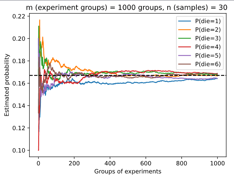
Wonder anyone has encountered the same problem as me related to the code above. In version 0.7 of Dive into Deep Learning, the code works as shown above, with all the probabilities converging to the expected value of 1/6. However, with code in version 0.8.0 of the same book, the curves (see the image on the right) do not look right. Both curves were obtained by running the code from the book(s) without any changes and ran on the same PC. So there might be bugs in version 0.8.0 of the book? Thanks!

1 reply
Jun '20 ▶ JohnG

StevenJokes

Maybe it is just a coincidence that almost 90 groups of experiments is “die = 6”?
It would be more clear if you counts / 1000 # Relative frequency as the estimate.

Jun '20

ness001

In L2/5 Naive Bayes, in terms of Nvidia Turing GPUs, why Alex said adding more silicons is almost free for Nvidia?

1 reply
Jun '20

goldpiggy

Hi @ness001, great question! Check here for more details about GPUs 13.4. Hardware — Dive into Deep Learning 1.0.3 documentation

Oct '20

alaa-shubbak

for question #3 can we calculate it like this :
P(A,B,C) = P(A/B,C) * P(B,C) and as B not depend on c
P(A,B,C) = P(A/B,C)*P(B)*P©
is it correct like this or not ? if not could you please explain why?
thanks in davaned

1 reply
Oct '20 ▶ alaa-shubbak

goldpiggy

Hey @alaa-shubbak, that’s correct!

Nov '20 ▶ StevenJokes

Aaron_L

For Q4:
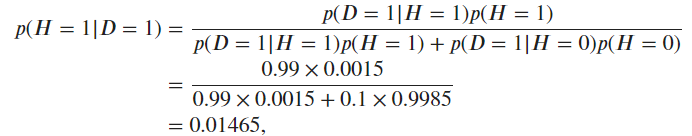
If we do the test 1 twice, the two tests won’t be independent, since they are using the same method on the same patient. In fact, we will get the same result very possibly.

Aug '21

zhenling

For Q3
P(ABC)=P(C|AB)P(AB)=P(C|B)P(B|A)P(A)
is it right? is it the simplest answer for Q3?

Mar '22

zgpeace

install fail

!pip install d2l==0.17.4

1 reply
Mar '22 ▶ zgpeace

HyunA_Kim

Can you try !pip install d2l, I succeeded, and where did you get this 0.17.4 version?

1 reply
Mar '22

zgpeace

It does work. I use pytorch in colab. Thank you so much.

May '22

Abhishek_Verma

In section 2.6.2.6
P(D1=1,D2=1) = P(D1=1,D2=1|H=0) * P(H=0) + P(D1=1,D2=1|H=1) * P(H=1)

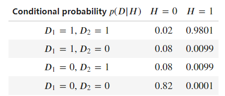
Is this equivalent to (since D1 and D2 are independent)
P(D1=1,D2=1) = P(D1=1) * P(D2=1) ?
P(D1=1) has been calculated in equation 2.6.3 and P(D2=1) can be calculated similarly.

I am having a hard time proving this. Am I missing something?

1 reply
May '22 ▶ Abhishek_Verma

Abhishek_Verma

“…by assuming the conditional independence”
my bad.

May '22

Tianrui_Zhang

Maybe there’s a typo in 2.6.7 which should be 0.00176655 and I have 0.8321304237 in 2.6.8. Correct?

Jun '22

MrBean

For the last question
If we assume the test result is deterministic, then

P(D2=1|D1=1) = 1
P(D2=0|D1=0) = 1

Doing first experiment twice does not add additional information. Therefore, P(H=1|D1=1,D2=1) == P(H=1|D1=1). You can derive the equation by doing some arithmetic.

Aug '22

timengler

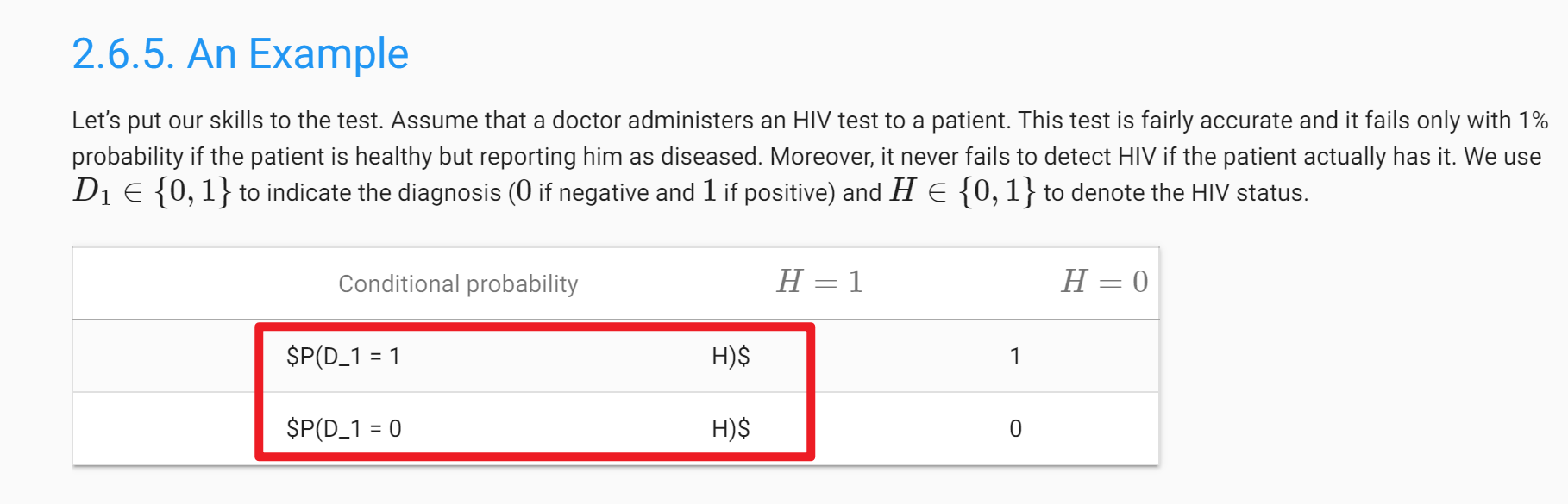
I don’t understand equation 2.6.3 . On the right side, why wouldn’t P(A) on the top cancel out with P(A) on the bottom, and since the other term on the bottom right which is the sum of all b in B for P(B|A) equals 1, wouldn’t that mean it would then just simplify to P(A|B) = P(B|A) which is obviously incorrect?

1 reply
Aug '22

Cesaryuan

There seems to be something wrong with the typesetting.

Aug '22 ▶ timengler

Gitartha_Kumar_Sarma

Yes, the equation is slightly wrong. The updated equation should sum over all possible ‘a’ values in the sample space(a and its complement so that it gets normalized accurately), Reference

Dec '22

Denis_Kazakov

An error in exercise 4? It says we draw n samples and then uses m in the definition of zm.

Jan '23

cajmorgan

Would have been great and more clear to actually see what numbers you multiplied in the example, for someone never doing stats before, it can be hard to comprehend all the formulas without any explanations.

Feb '23

tuntunia

Answer for Problem 7:
Part 1:

                        | P(D2=1|H=0) | P(D2=0|H=0) | Total
P(D1=1|H=0)	|               0.02	|               0.08 | 0.10
P(D1=0|H=0)	|               0.08	|               0.82	| 0.90
Total                |               0.10 |                0.90 | 1.00

Part 2:

P(H=1|D1=1) = P(D1=1|H=1) * P(D2=0|H=1) / P(D1=1)

P(D1=1) = P(D1=1,H=0) + P(D1=1, H=1)
=> P(D1=1) = P(D1=1|H=0) * P(H=0) + P(D1=1|H=1) * P(H=1)

Thus, P(H=1|D1=1) = (0.99 * 0.0015) / ((0.10 * 0.9985) + (0.99 * 0.0015)) = 0.01465

Part 3:

P(H=1|D1=1,D2=1) = P(D1=1,D2=1|H=1) * P(H=1) / P(D1=1,D2=1)                     (1)
P(D1=1,D2=1|H=1) = P(D1=1|H=1) * P(D2=1|H=1)                                               (2)
P(D1=1,D2=1) = P(D1=1,D2=1,H=0) + P(D1=1,D2=1,H=1)
                        = P(D1=1,D2=1|H=0) * P(H=0) + P(D1=1,D2=1|H=1) * P(H=1)     (3)
Using (1), (2), & (3),
P(H=1|D1=1,D2=1) = 0.99 * 0.99 * 0.0015 / (0.02 * 09985 + 0.99 * 0.99 * 0.0015) = 0.06857

Are the above answers correct??

3 replies
Feb '23

block_ramen

“For an empirical review of this fact for large scale language models see Revels et al. (2016).”

I believe this citation is wrong. It links to an auto-grad paper with nothing to do with evaluating LLMs.

Mar '23 ▶ tuntunia

Denis_Kazakov

I got the same answers independently. Now, we can try and calculate the probability of both of us being wrong.

Jun '23

SighingSnow

I have a qustion that, for the first problem of Q7 we have P(D1=1|H=0) = 0.1 but the condition listed above is P(D1=1|H=0) = 0.01 ?

1 reply
Jun '23 ▶ SighingSnow

Shawn_Shan

You need to read carefully, it states: P(D1=0|H=1) = 0.01 (false negative). P(D1=1|H=0) = 0.1 (False positive)

Jun '23 ▶ tuntunia

Shawn_Shan

Got the same results as well

Jul '23 ▶ tuntunia

cclj

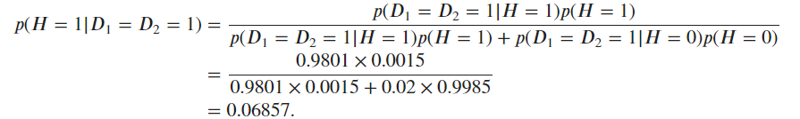
The same answer. Quite conterintuitive, though. I think it is because the joint FPR 0.02 increased a lot compared to the original example 0.0003. So the positive result can still be confusing to patients.

Jul '23

cclj

Ex3.

Ex7.

1 reply
Mar '24

kyunghee_cha

Q8-a)

Mar '24

kyunghee_cha

Q8-b)

Q8-c)

The weighting should be highest for stocks with the most highly expected return.

Mar '24

kyunghee_cha

Q8-d)

With no risk-free assets in a portfolio:

Please let me know if I am wrong.

Mar '24 ▶ cclj

Kaiwen_Xie

could i ask, for question 3, the variance, how did u get from the 2nd line to the 3rd line? I am a little stuck at that part

Aug '24

mayank64ce

Can someone explain the approaches to problems 3, 4, 6 and 8 ??

Oct '24

Nicolas_Victorion

Hi, I’m confused because it seems you are using “sample size” and “samples” interchangeably.

15 Jan

filipv

As a note for the authors, the citation of Revels et. al 2016 in 2.6.7 looks wrong. Maybe this was supposed to be Kaplan et al. 2020, or Hoffmann et al. 2022.

16 Jan

filipv

My answers to these exercises:

  1. Any entirely deterministic process - for example, determining the weight in kilograms of an arbitrary quantity of lithium.
  2. Any process with stochastic components - for example, predicting tomorrow’s stock prices. One can get to a certain point of accuracy if they closely follow news events and filings, and get good at modeling, but there’s always uncertainty as to the exact decisions others will make. One might argue against such processes existing on fatalist grounds!
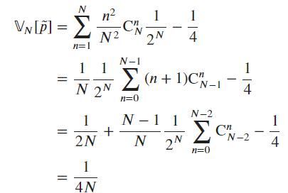
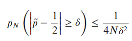
  3. The variance is equal to p*(1-p) / n. This means the variance scales with 1/n, where n is the number of observations. Using Chebyshev’s inequality, we can bound \hat{p} with P\left(|\hat p - p| \ge k \cdot \sqrt{\frac{p(1-p)}{n}}\right) \le \frac{1}{k^2} (with p=0.5 in our case, assuming the coin is fair). Chebyshev’s inequality gives us a distribution-free bound, but as n grows (typically for n > 30), the central limit theorem tells us that \hat p \approx \mathcal{N} \left(p, \frac{p(1-p)}{n}\right)
  4. I’m not sure if I’m interpreting the phrase “compute the averages” correctly, but I wrote the following snippet:
l = 100
np.random.randn(l).cumsum() / np.arange(1, l+1)

As for the second part of the question - Chebyshev’s inequality always holds for a single random variable with a finite variance. You can apply Chebyshev’s inequality to a specific z_m, but you cannot apply it for each z_m independently. This is because the z_ms are not i.i.d. - they share most of the same underlying terms!
5. For P(A \cup B), the lower bound is max(P(A), P(B)), and the upper bound is max(1, P(A) + P(B)). For P(A \cap B), the lower bound is max(0, P(A)+P(B)-1) (remember that P(A)+P(B) can be larger than 1) and the upper bound is min(P(A), P(B))
6. One could factor the joint probability P(A, B, C) as P(C|B) * P(B|A) * P(A), but this isn’t simpler. I’m not sure what exactly this question is looking for.
7. We know that the false positive rate for each test must add up to 0.1, and that the joint probabilities must add up to 1. So the mixed probabilities are 0.08, and P(D_1=0, D_2=0 | H=0) = 0.82. For 7.2, I obtained 1.47%. For 7.3, I obtained 6.86%.
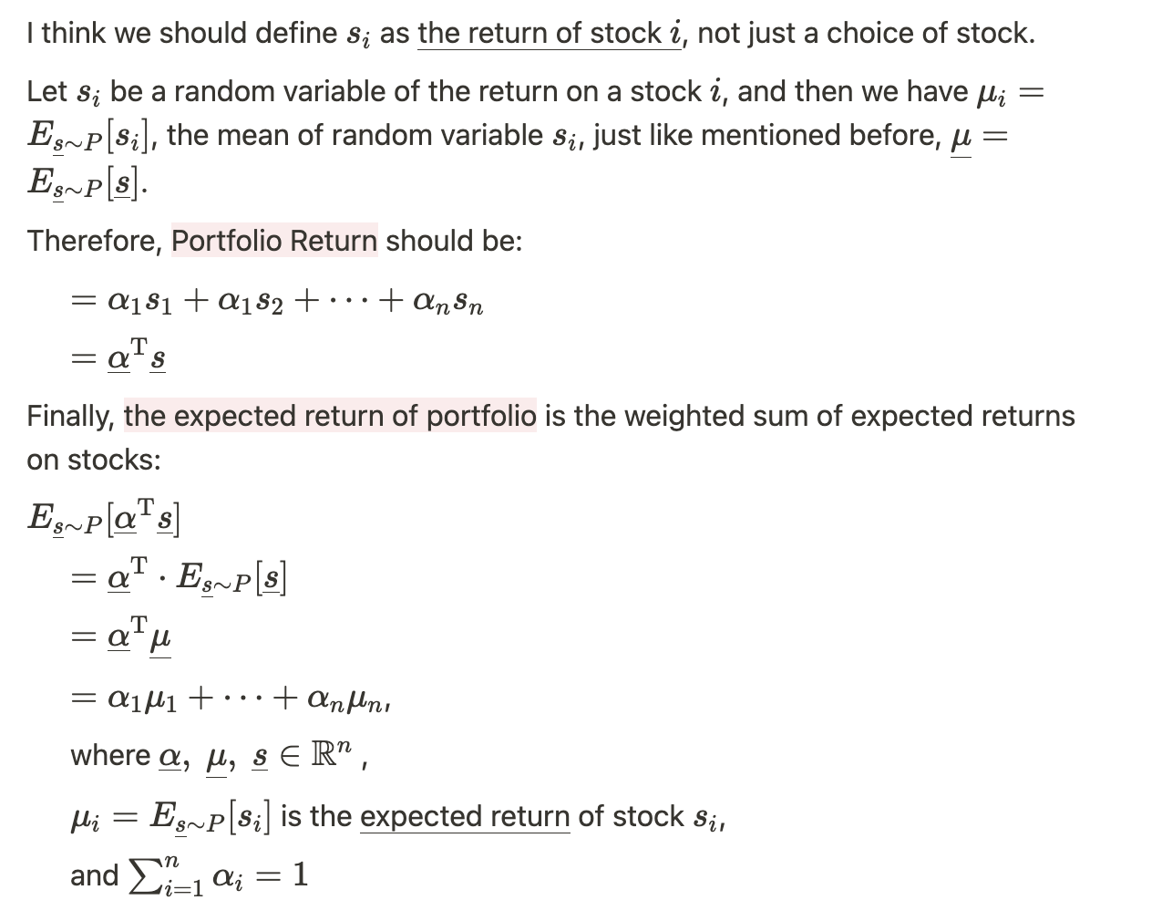
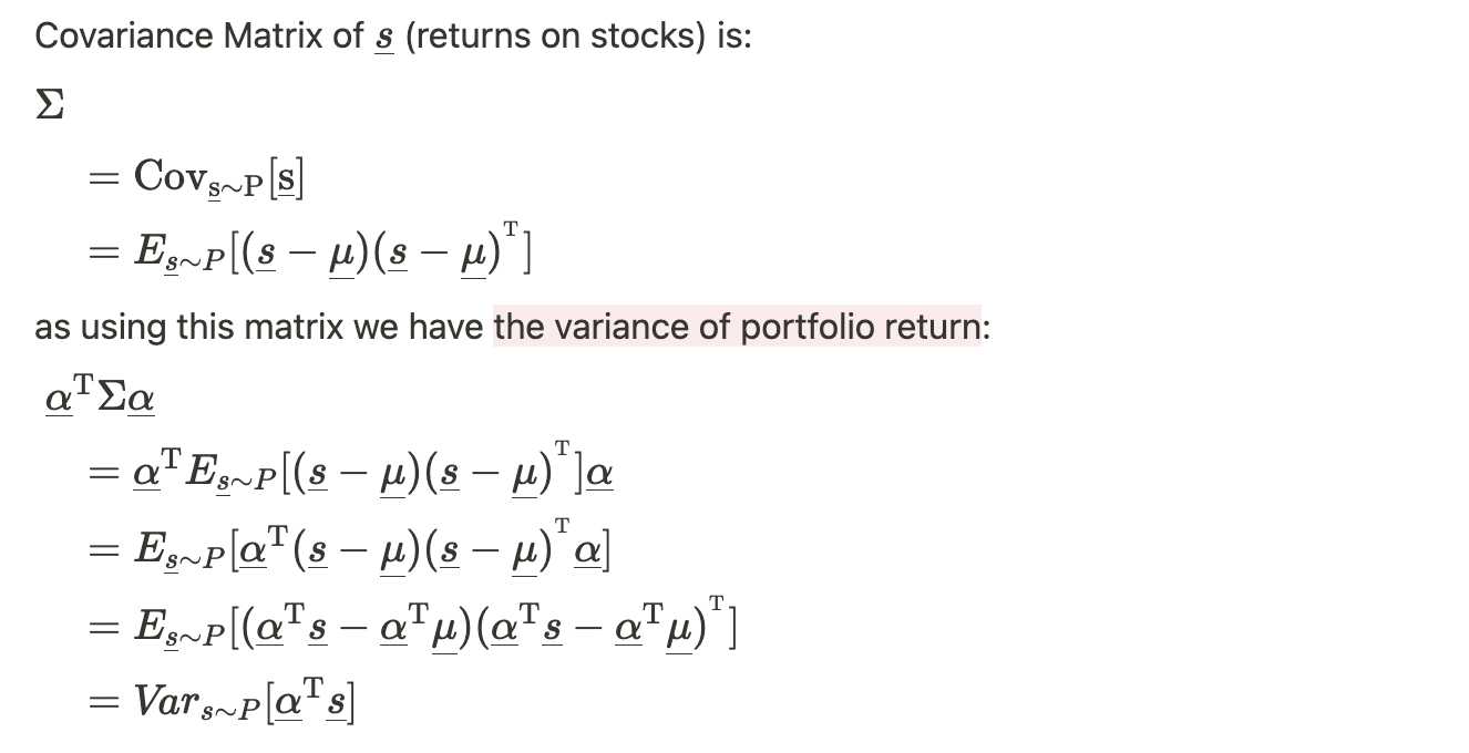
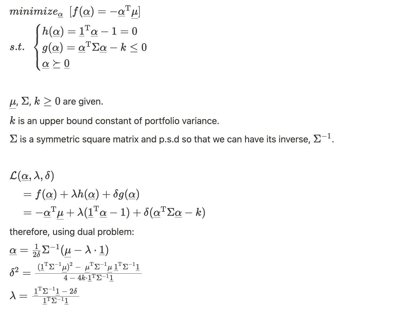
8. The expected return for a given portfolio \boldsymbol \alpha are \boldsymbol \alpha^\top \boldsymbol \mu. To maximize the expected returns of the portfolio, one should find the largest entry in \mu_i and invest the entire portfolio into it - \boldsymbol \alpha should have a single non-zero entry at the corresponding index. The variance of the portfolio is \boldsymbol \alpha^\top \Sigma \boldsymbol \alpha. So the optimization problem described can be formalized as: maximize \boldsymbol \alpha^\top \boldsymbol \mu for some maximum variance \boldsymbol \alpha^\top \Sigma \boldsymbol \alpha, where \sum_{i=1}^n \alpha_i = 1 and \alpha_i \ge 0.