Wonder anyone has encountered the same problem as me related to the code above. In version 0.7 of Dive into Deep Learning, the code works as shown above, with all the probabilities converging to the expected value of 1/6. However, with code in version 0.8.0 of the same book, the curves (see the image on the right) do not look right. Both curves were obtained by running the code from the book(s) without any changes and ran on the same PC. So there might be bugs in version 0.8.0 of the book? Thanks!
Maybe it is just a coincidence that almost 90 groups of experiments is “die = 6”?
It would be more clear if you counts / 1000 # Relative frequency as the estimate.
For Q4:
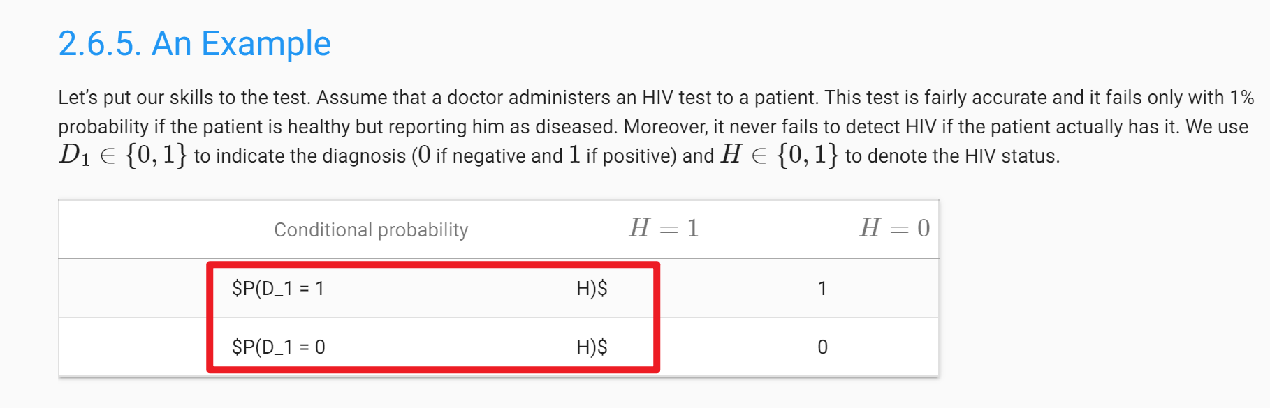
If we do the test 1 twice, the two tests won’t be independent, since they are using the same method on the same patient. In fact, we will get the same result very possibly.
Is this equivalent to (since D1 and D2 are independent) P(D1=1,D2=1) = P(D1=1) * P(D2=1) ? P(D1=1) has been calculated in equation 2.6.3 and P(D2=1) can be calculated similarly.
I am having a hard time proving this. Am I missing something?
For the last question
If we assume the test result is deterministic, then
P(D2=1|D1=1) = 1
P(D2=0|D1=0) = 1
Doing first experiment twice does not add additional information. Therefore, P(H=1|D1=1,D2=1) == P(H=1|D1=1). You can derive the equation by doing some arithmetic.
I don’t understand equation 2.6.3 . On the right side, why wouldn’t P(A) on the top cancel out with P(A) on the bottom, and since the other term on the bottom right which is the sum of all b in B for P(B|A) equals 1, wouldn’t that mean it would then just simplify to P(A|B) = P(B|A) which is obviously incorrect?
Yes, the equation is slightly wrong. The updated equation should sum over all possible ‘a’ values in the sample space(a and its complement so that it gets normalized accurately), Reference