StevenJokes

x = np.arange(0, 3, 0.1)
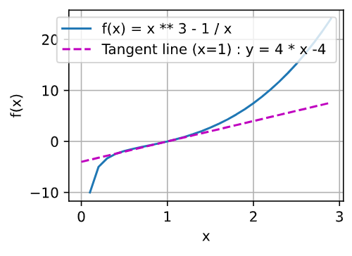
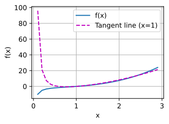
plot(x, [x ** 3 - 1 / x, 4 * x - 4], 'x', 'f(x)', legend=['f(x) = x ** 3 - 1 / x ', 'Tangent line (x=1) : y = 4 * x - 4 '])

According to the power rule and multiple rule," 3 * x ** 2 + 1 / (x ** 2) "is the derivative function of f (x).

So x == 1,f’(1) ==3 * 1 **2 + 1 / (1 ** 2) == 3 + 1 == 4,tangent line’s slope is 4.

And we know, the tangent line passes the plot (1, 0).

So the function of the line is " y == 4 * (x - 1) == 4 * x -4"

---

I have some problem with saving the “plot” picture, so I just screenshoted it.

I can still remember it is easy to save other “plot” pictures (eg. Statsmodel)by double-clicking the pic and clicking the “save” botton in VScode.

Is there a way to save instead of screenshoting ?

2 replies

goldpiggy

Hi @StevenJokes! Here is a hint you can try!
https://matplotlib.org/3.1.0/api/_as_gen/matplotlib.pyplot.savefig.html

StevenJokes

Is there a way to open it in VScode?
Or how to make it openable in VScode?

The doc is not friendly to other users.
https://matplotlib.org/3.1.0/api/_as_gen/matplotlib.pyplot.savefig.html

anandsm7

Hi,

Thanks for the great content guys
but i feel like giving examples in gradients and chain rule would be really helpful
Thanks

2 replies

goldpiggy

Hi @anandsm7, the gradients and chain rule are in section http://d2l.ai/chapter_appendix-mathematics-for-deep-learning/multivariable-calculus.html#multivariate-chain-rule. Feel free to do a search in the top right of our wensite as here:

StevenJokes

some apis:

1. plt.gca

---

Get the current Axes instance on the current figure matching the given keyword args, or create one.

Examples:

To get the current polar axes on the current figure:

plt.gca(projection='polar')

If the current axes doesn’t exist, or isn’t a polar one, the appropriate axes will be created and then returned.

---

https://matplotlib.org/3.1.1/api/_as_gen/matplotlib.pyplot.gca.html

---

2. axes.cla()

‘’’
Clear an axes, i.e. the currently active axes in the current figure. It leaves the other axes untouched.
‘’’

---

https://matplotlib.org/api/pyplot_api.html#matplotlib.pyplot.cla.

---

3. fmts:

• ‘-’:solid line style 实线;
• ‘m–’:magenta dashed line style 紫红色虚线;
• ‘g-’:green dash-dotted line style 绿色点划线；
• 'r:'red dotted line style 红色点线

---

For more:

1. https://blog.csdn.net/leaf_zizi/article/details/87094168
2. https://matplotlib.org/api/_as_gen/matplotlib.axes.Axes.plot.html#matplotlib.axes.Axes.plot
3. https://matplotlib.org/api/_as_gen/matplotlib.lines.Line2D.html#matplotlib.lines.Line2D.set_linestyle

akhil_teja

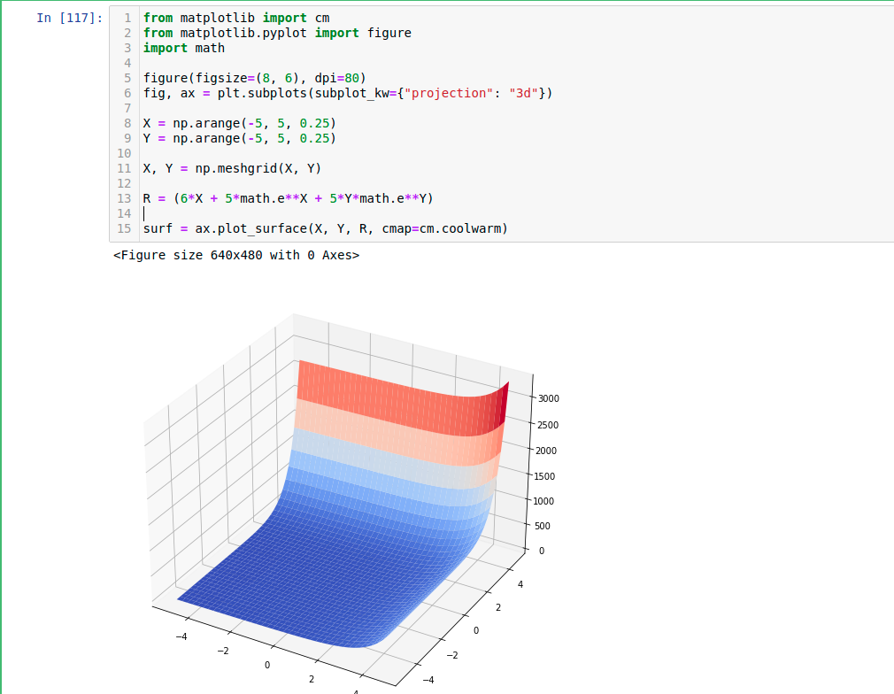
For the 2nd question in Excercises. Do we have different variables x1 and x2 or is it a single variable x ? If it’s a single variable, is it 5ex^2 that is in the equation?

1 reply

goldpiggy

Hi @akhil_teja, the x is a vector, i.e. x = [x1, x2]^T

rammy_vadlamudi

Hi does D2L provide a way where we can validate or check our solutions for the exercises ?

2 replies

StevenJokes

Discussion is the only way now.
@rammy_vadlmudi

goldpiggy

Hey @rammy_vadlamudi, yes! This discussion forum is great way to share your thoughts and discuss the solutions. Feel free to voice it out!

Luis_Ramirez

Hey guys hope u all good. I’ve found today this course. It’s quite interesting. I’m completing it in python. I’m learning mostly python for machine learning and AI applications. Even i’ve been learning how to manage to use AWS sagemaker and clouds services. But i wanted to ask a question about finding the gradient of the function. I mean question 2: It’s possible to define
a function like
import numpy as np
def(x): where x is a list
return 3x[0]**2 + 5np.exp(x[1])
and then apply numerical_limit function with following parameters(f = f(x), x =[1,1], h =0.01)
and return a list looping thought each index of the list x =[1,1]
or this logic is too dump?
If you guys can help me
I studied math in the past, but don’t know how to code with the most fresh and efficient way x)

thanks in advance

2 replies

goldpiggy

Hi @Luis_Ramirez, your logic is never dump! In most of DL framework, we decompose a complex function to each directly differentiable step and then apply the chain rule (i,e., we define all the derivative formula in code and apply chain rule). Check https://d2l.ai/chapter_preliminaries/autograd.html for more details. Besides, if you would like to see how to code from scratch, check here. Let me know if it helps!

Diachrony

Try adding this line to the top of the plot function:

fig = d2l.plt.figure() 

and have the plot function

return fig

then:

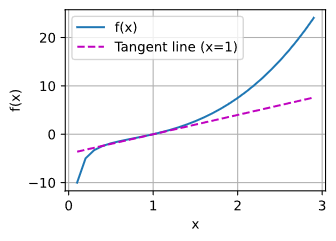
def f(x)
    return(x**3-1/x)
x = np.arange(0.1, 3, 0.1)
fig = plot(x, [f(x), 4 * x-4], 'x', 'f(x)', legend=['f(x)', 'Tangent line (x=1)'])

fig.savefig("2_Prelim 4_Calc 1_Ex.jpg")

ufs

• Q1
  

Amalia

hello,
I tried my code:
import torch
x = torch.arange(2.0)
x.requires_grad_(True)
x.grad
y = 3 * torch.dot(x,x) + 5 * torch.exp(x)
y
y.backward()
x.grad

¿it’s ok?

t1dumsharjah

Hi, I’m looking for some clarification on this excerpt from the very end of Section 2.4.3:

Similarly, for any matrix 𝐗, we have ∇𝐗 ‖𝐗‖_F^2 = 2𝐗.

Does this mean that for a given matrix of any size filled with m*n variables, the gradient of the square of that matrix can be condensed to 2X?

Also, what does the subscripted F imply in this case?

Thanks!

1 reply

t1dumsharjah

Hi, I just wanted to verify my solutions for the provided exercise questions:

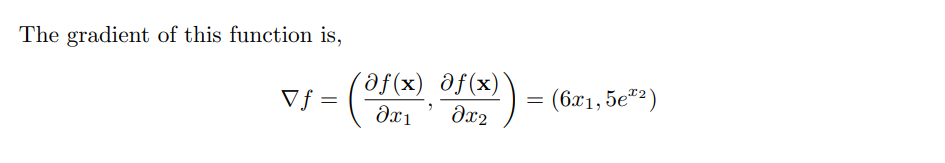
1. Find the gradient of the function 𝑓(𝐱)=3*(𝑥1 ^ 2) + 5𝑒^𝑥2

(Subsituting y for x2, as I assumed x1 != x2)

f’(x) = 6x + 5e^y

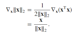
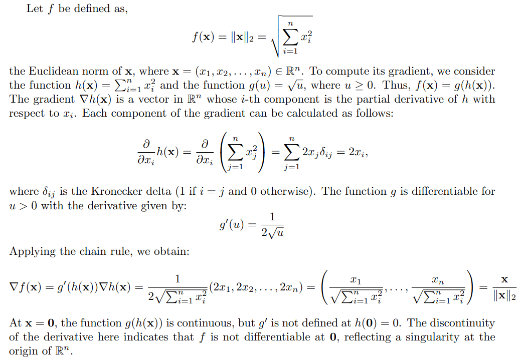
2. What is the gradient of the function 𝑓(𝐱)=‖𝐱‖2

||x||2 = [ (3x^2)^2 + (5e^y)^2 ]^0.5

(Calculating the Euclidean distance using the Pythagorean Theorem)

||x|| = ( 9x^4 + 25e^2y ) ^ 0.5

f’ ( ||x|| ) = ( 18x^3 + 25e^2y ) / ( 9x^4 + 25e^2y ) ^ 0.5

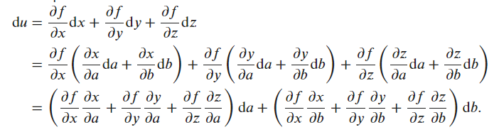
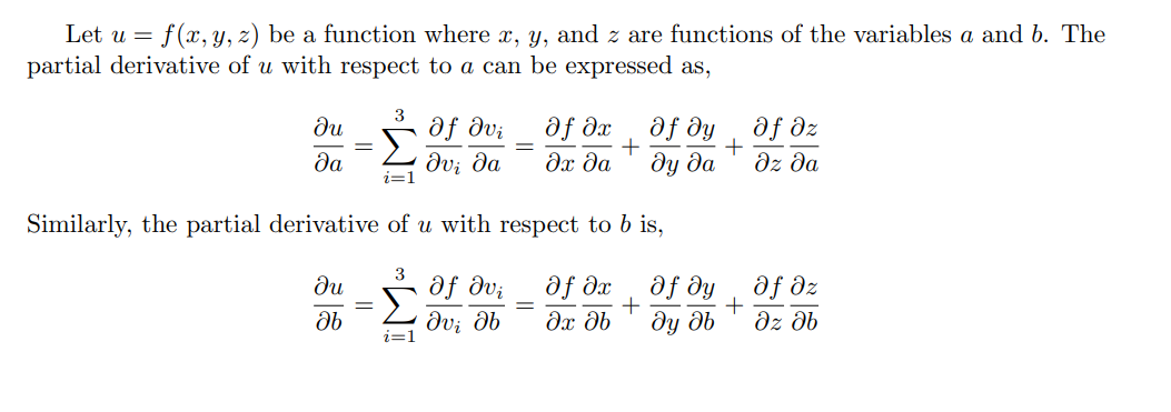
4. Can you write out the chain rule for the case where 𝑢=𝑓(𝑥,𝑦,𝑧), 𝑥=𝑥(𝑎,𝑏), 𝑦=𝑦(𝑎,𝑏), and 𝑧=𝑧(𝑎,𝑏)?

Is this meant to be simplified to df/dx * (dx/da + dx/db) and so on for y, and z?

Thanks so much, and I apologise if my answers are completely misguided.

VolodymyrGavrysh

2. Find the gradient of the function f (x) = 3x12 + 5ex2

x1/df = 6x + 5e^x2
x2/df = 52e^x2

∇ x f (x) = [6x + 5ex2, 52ex2]

here is pic (not sure if it’s correct)

1 reply

xela21co

I’m confused with partial derivatives. Since for partial derivatives we can treat all other variables as constants, shouldn’t the derivative vector be [6x_1, 5e^x_2] ?

∂f/∂x_1 = ∂/∂x_1 (3x_1^2) + DC = 6x_1 + 0 = 6x_1 (C being a constant)
∂f/∂x_2 = DC + ∂/∂x_2 (5e^x_2) = 0 + 5e^x_2 = 5e^x_2

xela21co

I believe the F implies the Frobenius Norm:
http://d2l.ai/chapter_preliminaries/linear-algebra.html?highlight=norms

I’m not clear on what the notation implies when there is both a subscript F and a superscript 2. The text reads as if the Frobenius Norm is always the square root of the sum of its matrix elements, so the superscript should always be 2. Is this understanding incorrect?

1 reply

pbouzon

Exercise 2:
∇f(x) = [6x1, 5e^x2]

Exercise 3:
f(x) = (x1² + x2² … + xn²)¹/²
∇f(x) = x/f(x)

Exercise 4:
u = f(x,y,z), x = x(a,b), y = y(a,b), z = z(a,b)

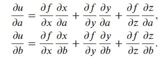
du/da = (du/dx)(dx/da) + (du/dy)(dy/da) + (du/dz)(dz/da)
du/db = (du/dx)(dx/db) + (du/dy)(dy/db) + (du/dz)(dz/db)

imflash217

The superscript 2 means you are squaring the Forbenius Norm. So, the square root in the Forbenius Norm disappears.

zgpeace

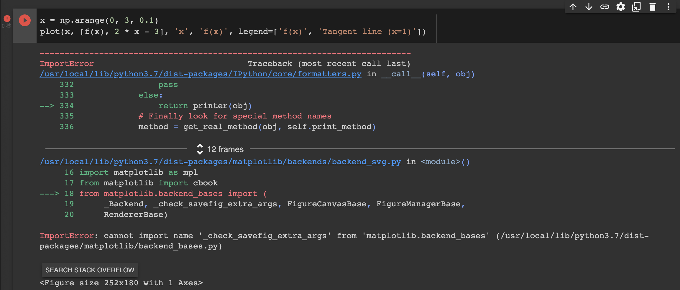
I found some issue, while I run the below code in pytorch.

    x = np.arange(0, 3, 0.1)
    plot(x, [f(x), 2 * x - 3], 'x', 'f(x)', legend=['f(x)', 'Tangent line (x=1)'])

1 reply

anirudh

Thanks @zgpeace for raising this, I believe it was recently deprecated but shouldn’t error out. You can try with an older version of ipython. In any case we’ll fix this in the next release https://github.com/d2l-ai/d2l-en/pull/2065

1 reply

zgpeace

Thank you @anirudh. I try to install d2l without version. !pip install d2l It works.

MrBean

For question one:

def f(x):
    return x ** 3 - 1.0 / x

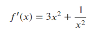
def df(x):
    return 3 * x ** 2 + 1/ (x * x)

def tangentLine(x, x0):
    """x is the input list, x0 is the point we compute the tangent line"""
    y0 = f(x0)
    a = df(x0)
    b = y0 - a * x0
    return a * x + b

x = np.arange(0.1, 3, 0.1)
plot(x, [f(x), tangentLine(x, 2.1)], 'x', 'f(x)', legend=['f(x)', 'Tangent line (x=2.1)'])

bit-scientist

the calculus.ipynb notebook kernel dies each time I run:

x = np.arange(0, 3, 0.1)
plot(x, [f(x), 2 * x - 3], 'x', 'f(x)', legend=['f(x)', 'Tangent line (x=1)'])

What am I supposed to do here? Thanks

donny_nyc

9. Would the idea be to use a ‘generalized’ chain rule and express du/da, and du/da (something like the gradient)

du/da = f’(dx/a) + f’(dy/da) + f’(dz/da)
du/db = f’(dx/db) + f’(dy/db) + f’(dz/db)

Maxim

tx = 3 * x ** 2 + (1 / x ** 2) - 4
plot(x, [f(x), tx], ‘x’, ‘f(x)’, legend=[‘f(x)’, ‘Tangent line (x=1)’])

1 reply

Denis_Kazakov

In section 2.4.3, you define gradient of a multivariate function assigning vector x to a scalar y.

At the end of the section, you give rules for gradients of matrix-vector products (which are matrices, not scalars).

I think it would help to define gradient of a matrix.

cajmorgan

I agree with this, felt like these big topics just got skipped over

aniketvp24

if x is a n dimensional column vector, so x is n by 1, so its transpose is 1 by n and dimension of A is m by n how is x_transpose.A possible then?

1 reply

cclj

Ex4.

• The function is not in the form of any rules given up to now.
  • Taking the logarithm on both sides yields
    

Ex5.

• Any point such that indicates a stationary point of a function, where a “ball” standing on the point will hold its position and will not fall along the curve.
  • The stationary point is necessary for a point to be a minimum or maximum point. Sometimes it indicates the critical behavior of a function.
• Example: at

Ex6.

• The derivative
  
  takes value 4 at point 1.
  • The tangent line at point 1 is thus

f = lambda x: x ** 3 - 1 / x
x = np.arange(0, 3, 0.1)
plot(x, [f(x), 4 * x - 4], 'x', 'f(x)', legend=['f(x)', 'Tangent line (x=1)'])

Output:

cclj

Ex7.

• The gradient is a 2D vector
  

Ex8.

• According to the chain rule,
  
• At , the derivative is not well-defined, since

Ex9.

• To make things clear, we perform a hierarchical expansion of the total differential.
  
  
• Therefore we have
  

GoM

Thanks for a great course!

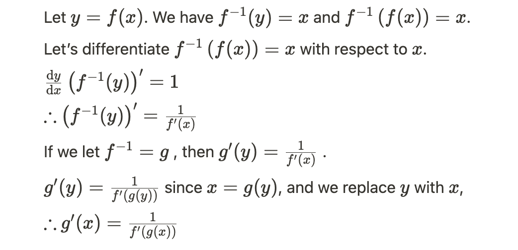
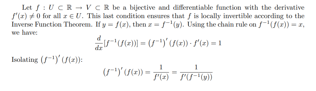
Any idea regarding Q10?

I used the given definitions as hinted - denote g=f^(-1), I was able to derive that

\frac{dg}{dx} = \frac{\frac{dg}{df}\frac{df}{dx}}{\frac{df}{dg}}

Is that the expected solution?
Thanks!

kyunghee_cha

I think the answer of Q10 is…

filipv

This forum won’t let me upload a pdf – if you’re interested in looking at my solutions, you’ll have to compile the LaTeX below.

\documentclass{article}
\usepackage{amsmath}
\usepackage{amssymb}

\begin{document}

\section*{Problem 1}

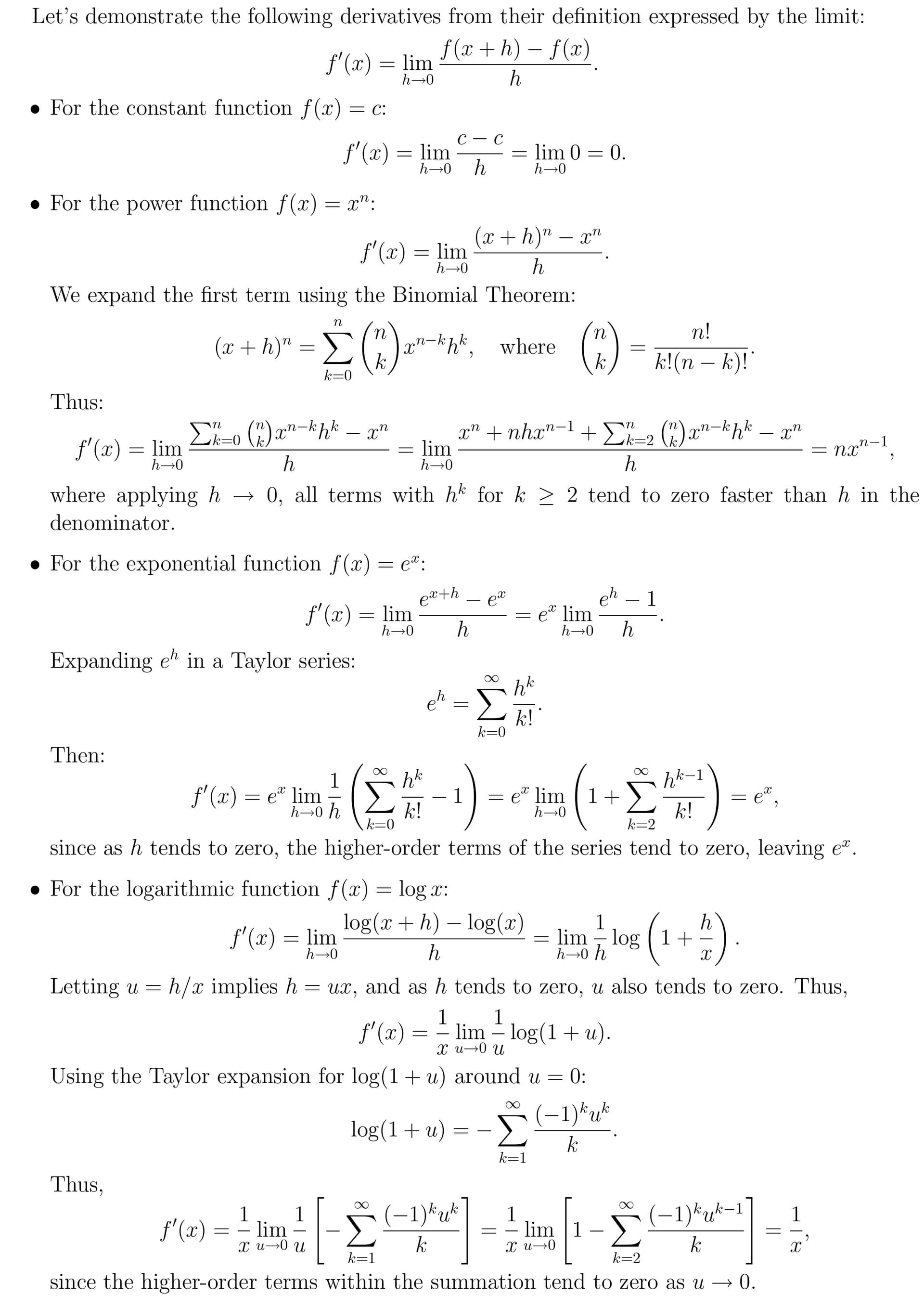
For $f(x) = c$ where $c$ is a constant, we have

$$
\lim_{h \to 0} \frac{f(x + h) - f(x)}{h} = \lim_{h \to 0} \frac{c - c}{h} = 0
$$

For $f(x) = x^n$, we have

\begin{equation}
\begin{split}
  \frac{df}{dx} &= \lim_{h \to 0} \frac{(x + h)^n - x^n}{h} \\ 
  &= \lim_{h \to 0} \frac{\binom{n}{0}x^nh^0 + \binom{n}{1}x^{n-1}h^1 + \binom{n}{2}x^{n-2}h^2 + \cdots - x^n}{h} \text{ via the binomial expansion} \\
  &= \lim_{h \to 0} \binom{n}{1}x^{n-1}h^0 + \binom{n}{2}x^{n-2}h^1 + \cdots \text{ after cancelling $x^n$ and dividing by $h$} \\
  &= \boxed{nx^{n-1}} \text{ since all terms with $h$ approach 0} \\
\end{split}
\end{equation}

For $f(x) = e^x$, we have

\begin{equation}
\begin{split}
  \frac{df}{dx} &= \lim_{h \to 0} \frac{e^{x + h} - e^x}{h} \\
  &= \lim_{h \to 0} \frac{e^xe^h - e^x}{h} \\
  &= \lim_{h \to 0} \frac{e^x(e^h - 1)}{h} \\
  &= e^x \times \lim_{h \to 0} \frac{e^h - 1}{h} \\
  &= e^x \times 1 \text{by L'Hopital's rule} \\
  &= \boxed{e^x} \\
\end{split}
\end{equation}

For $f(x) = \log(x)$

\begin{equation}
\begin{split}
  \frac{df}{dx} &= \lim_{h \to 0} \frac{\log(x + h) - \log(x)}{h} \\
  &= \lim_{h \to 0} \frac{\log\left(\frac{x + h}{x}\right)}{h} \\
  &= \lim_{u \to 0} \frac{\log\left(1 + u\right)}{ux} \text{ with } u = \frac{h}{x} \\
  &= \frac{1}{x} \lim_{u \to 0} \frac{\log(1 + u)}{u} \\
  &= \frac{1}{x} \lim_{u \to 0} \frac{1}{(1 + u)\ln{10}} \text{ by L'Hopital's rule} \\
  &= \boxed{\frac{1}{x\ln{10}}} \\
\end{split}
\end{equation}

This proof is a bit circular since it uses the derivative of $\log(x)$ when applying L'Hopital's rule! If you found a better proof, let me know.

\section*{Problem 2}

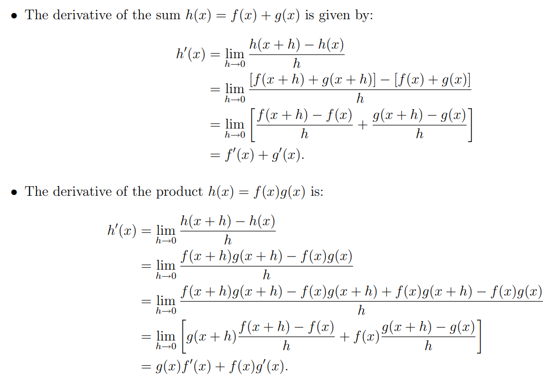
For the product rule:

\begin{equation}
\begin{split}
&\text{Prove } \frac{d}{dx} \left[ f(x)g(x) \right] = f(x)g'(x) + g(x)f'(x) \\
&= \lim_{h \to 0} \frac{f(x+h)g(x+h) - f(x)g(x)}{h} \text{ using the definition of a derivative} \\
&= \lim_{h \to 0} \frac{f(x+h)g(x+h) - f(x+h)g(x) + f(x+h)g(x) - f(x)g(x)}{h} \\
&= \lim_{h \to 0} \frac{f(x+h)\left[g(x+h)-g(x)\right] + g(x)\left[f(x+h)-f(x)\right]}{h} \\
&= f(x+0)\lim_{h \to 0} \frac{g(x+h)-g(x)}{h} + g(x)\lim_{h \to 0} \frac{f(x+h)-f(x)}{h} \\
&= \boxed{f(x)g'(x) + g(x)f'(x)} \\
\end{split}
\end{equation}

For the sum rule:

\begin{equation}
\begin{split}
&\text{Prove } \frac{d}{dx} \left[ f(x)+g(x) \right] = f'(x) + g'(x) \\
&= \lim_{h \to 0} \frac{[f(x+h)+g(x+h)] - [f(x)+g(x)]}{h} \\
&= \lim_{h \to 0} \frac{f(x+h) - f(x)}{h} + \lim_{h \to 0} \frac{g(x+h) - g(x)}{h} \\
&= \boxed{f'(x) + g'(x)} \\
\end{split}
\end{equation}

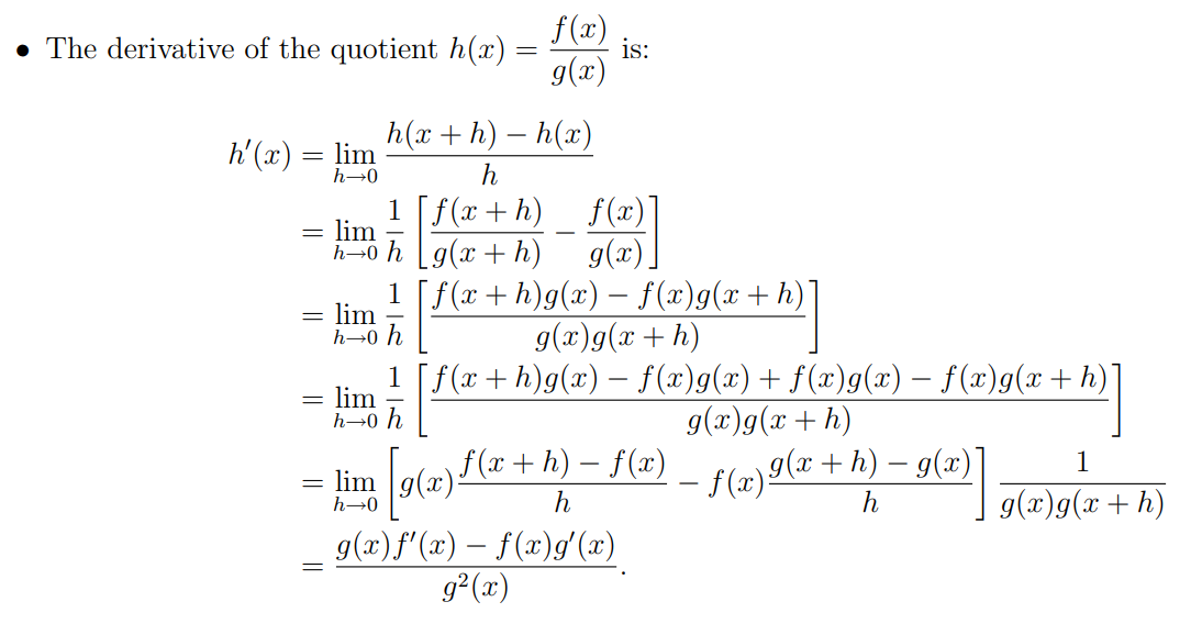
For the quotient rule:

\begin{equation}
\begin{split}
&\text{Prove } \frac{d}{dx} \left( \frac{f(x)}{g(x)} \right) = \frac{g(x)f'(x) - f(x)g'(x)}{g^2(x)} \\
&= \lim_{h \to 0} \frac{\frac{f(x+h)}{g(x+h)} - \frac{f(x)}{g(x)}}{h} \\
&= \lim_{h \to 0} \frac{f(x+h)g(x) - f(x)g(x+h)}{hg(x)g(x+h)} \\
&= \lim_{h \to 0} \frac{f(x+h)g(x)-f(x)g(x)+f(x)g(x)-f(x)g(x+h)}{hg(x+h)g(x)} \\
&= \lim_{h \to 0} \frac{g(x)[f(x+h)-f(x)] - f(x)[g(x+h)-g(x)]}{hg(x)g(x+h)} \\
&= \boxed{\frac{f'(x)g(x) - f(x)g'(x)}{g(x)^2}} \\
\end{split}
\end{equation}

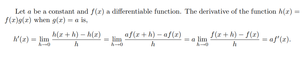
\section*{Problem 3}

The product rule states $\frac{d}{dx}[f(x)g(x)] = f(x)g'(x) + g(x)f'(x)$. Let $g(x) = c$.

$$
f(x)\frac{d}{dx}c + c\frac{d}{dx}f(x) = f(x)\cdot0 + c\frac{d}{dx}f(x) = \boxed{c\frac{d}{dx}f(x)}
$$

\section*{Problem 4}

\begin{equation}
\begin{split}
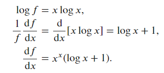
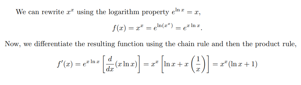
y &= x^x \\
\ln{y} &= \ln{x^x} = x\ln{x} \\
\frac{1}{y}\cdot\frac{dy}{dx} &= \ln{x} + x \cdot \frac{1}{x} \text{ by the product rule} \\
\frac{dy}{dx} &= y(\ln{x} + 1) \\
\frac{dy}{dx} &= x^x(\ln{x} + 1) \\
\end{split}
\end{equation}

\section*{Problem 5}

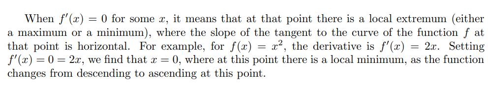
$f(x)$ has a slope of 0 at that point. For instance, $f(x) = x^2$ has a slope of 0 at $x = 0$.

\section*{Problem 6}

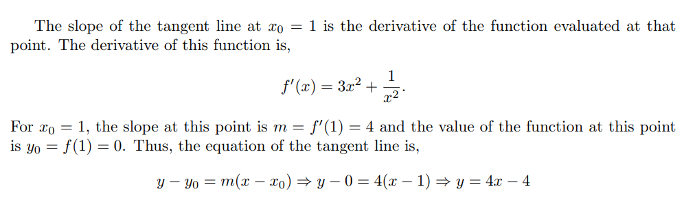
Done using $3x^2 + \frac{1}{x^2}$ to calculate the slope, yielding the final equation $4x-4$.

\section*{Problem 7}

$$
\nabla_x f(x) =
\begin{bmatrix}
  6x_1 \\
  5e^{x_2} \\
\end{bmatrix}
$$

\section*{Problem 8}

\begin{equation}
\begin{split}
  f(\mathbf{x}) &= \|\mathbf{x}\|_2 \\
  \nabla_{\mathbf{x}} \|\mathbf{x}\|_2 &= \nabla_{\mathbf{x}} (\mathbf{x}^{\top}\mathbf{x})^{1/2} \\
  &= 2\mathbf{x} \cdot \frac{1}{2}(\mathbf{x}^{\top}\mathbf{x})^{-1/2} \\
  &= \boxed{\frac{\mathbf{x}}{\|\mathbf{x}\|_2}} \\
\end{split}
\end{equation}

At $x=0$, the gradient is undefined.

\section*{Problem 9}

$$
\frac{\partial{u}}{\partial{a}} = \frac{\partial{u}}{\partial{x}} \cdot \frac{\partial{x}}{\partial{a}} + \frac{\partial{u}}{\partial{y}} \cdot \frac{\partial{y}}{\partial{a}} + \frac{\partial{u}}{\partial{z}} \cdot \frac{\partial{z}}{\partial{a}}
$$

\section*{Problem 10}

\begin{equation}
\begin{split}
y &= f^{-1}(x) \\
x &= f(y) \\
1 &= f'(y) \cdot \frac{dy}{dx} \\
\frac{dy}{dx} &= \frac{1}{f'(y)} \\
\frac{d}{dx}f^{-1}(x) &= \frac{1}{f'(f^{-1}(x))} \\
\end{split}
\end{equation}

\end{document}

1 reply

Sarah

Exercise 1

• Taylor expansion for e^h: WolframAlpha, and for log(1 + u): WolframAlpha.

Exercise 2

Exercise 3

Exercise 4

Exercise 5

Exercise 6

import numpy 
import matplotlib.pyplot as plt

# Code omitted to make the graph look nice: `plt.rcParams.update...`

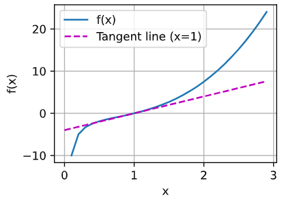
def f(x):
    return x ** 3 - 1 / x

def df(x):
    return 3 * x ** 2 + 1 / x ** 2

def tangent(x, x_0):
    return df(x_0) * (x - x_0) + f(x_0)

x_0 = 1 
x = np.arange(0.01, 2, 0.01) 

_, ax = plt.subplots()
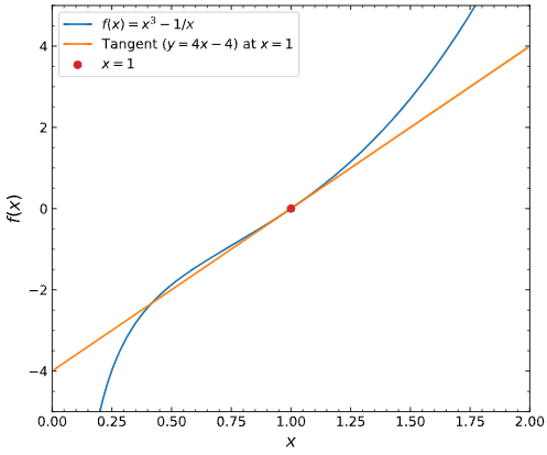
ax.plot(x, f(x), label="$f(x) = x^3 - 1/x$") 
ax.plot(x, tangent(x, x_0), label="Tangent $(y = 4x - 4)$ at $x=1$")
ax.scatter(x_0, tangent(x_0, x_0), zorder=10, color="tab:red", label="$x=1$") 
ax.set(xlabel="$x$", ylabel="$f(x)$", xlim=(0, 2), ylim=(-5, 5))
ax.legend();

Exercise 7

Exercise 8

Exercise 9

Exercise 10

Source: Inverse function theorem.

dhruvadeep_malakar

your tangent is a line, but your graph shows a curve. Tangent Line is defined as mx+c where m is the slope and c is a constant.

filipv

Revisiting this chapter, I remember being confused by the orientation of the gradients listed in section 2.4.3 – as a hint for other readers, I recommend reading the Layout conventions section of the Matrix calculus Wikipedia Article. This textbook’s appendix, specifically section 22.4.7 is also a great resource.

To summarize, there are two popular conventions for vector-vector derivatives:

1. In the numerator-based layout (sometimes called the Jacobian layout), the derivative has the same number of rows as the numerator’s dimensionality.
2. In denominator-based layouts (sometimes called the Hessian or gradient layout), the derivative has the same number of rows as the denominator’s dimensionality. This is sometimes notated by using a gradient symbol, as the authors do here. You also sometimes see a transpose symbol in the denominator to hint the reader that the denominator-based layout is being used.

wsehjk

This seems to be an error.
should be
.
I have created an issue to talk about this

rdong8

In 2.4.10, is $$\mathbf A$$ the Jacobian?