pbouzon
November 8, 2021, 10:11pm
23
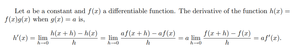
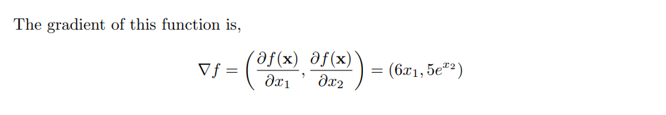
Exercise 2:x ) = [6x1, 5e^x2]
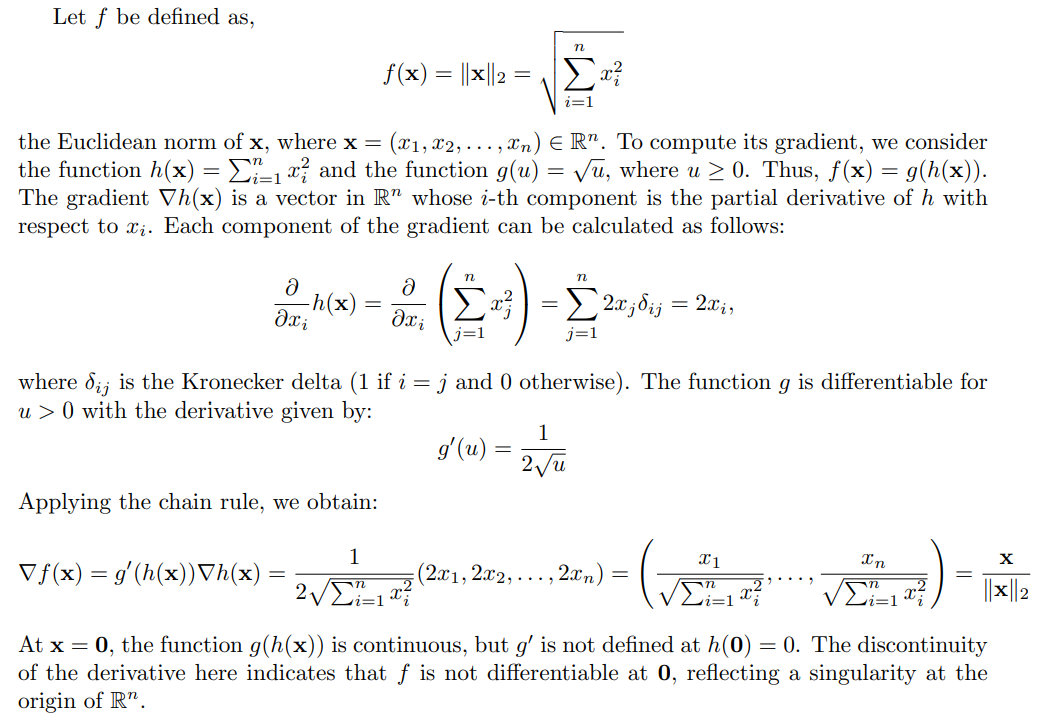
Exercise 3:x ) = (x1² + x2² … + xn²)¹/²x ) = x /f(x )
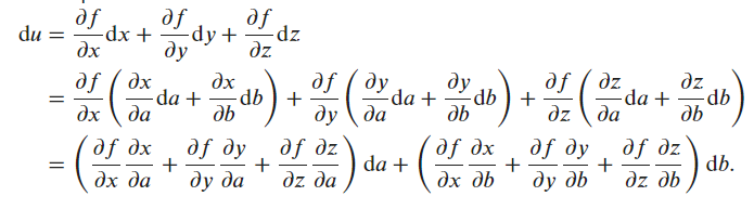
Exercise 4:
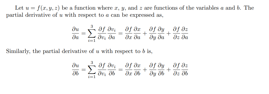
du/da = (du/dx)(dx/da) + (du/dy)(dy/da) + (du/dz)(dz/da)
2 Likes
The superscript 2 means you are squaring the Forbenius Norm. So, the square root in the Forbenius Norm disappears.
I found some issue, while I run the below code in pytorch.
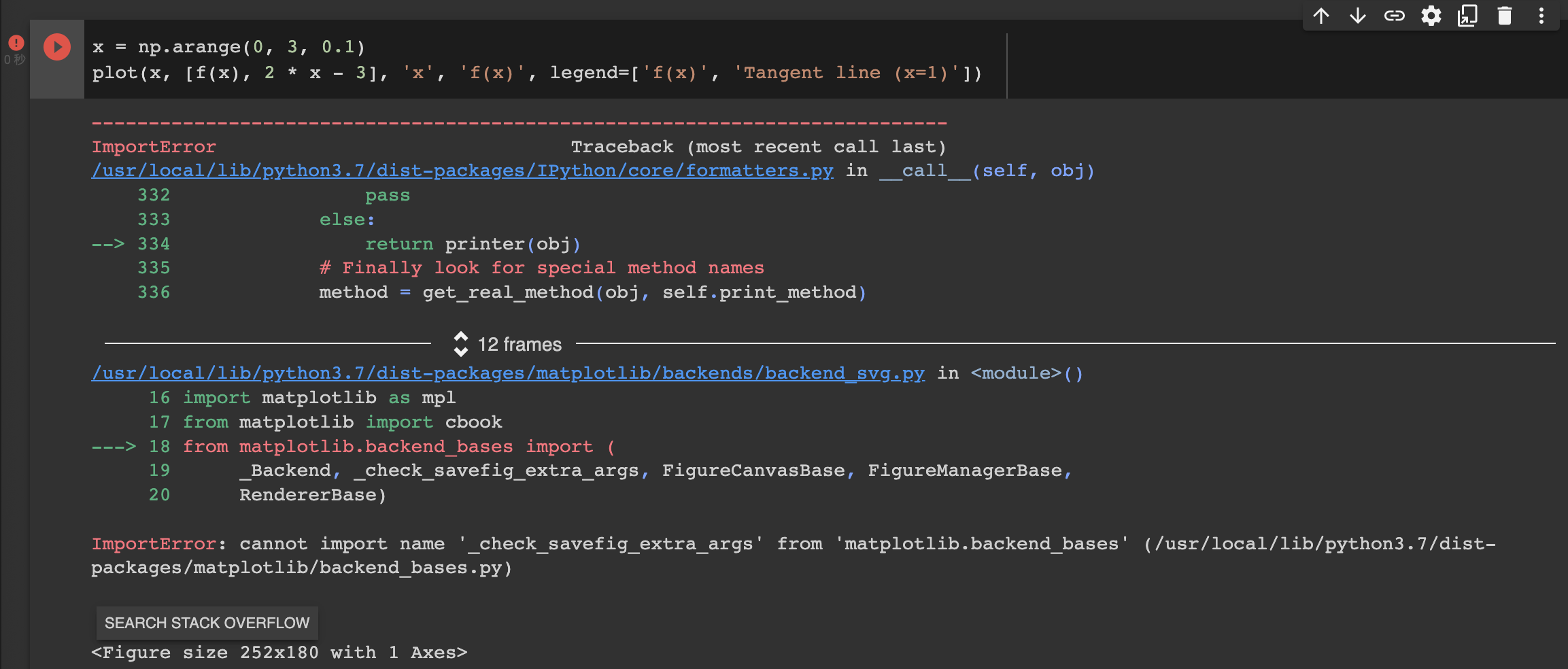
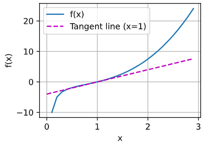
    x = np.arange(0, 3, 0.1)
    plot(x, [f(x), 2 * x - 3], 'x', 'f(x)', legend=['f(x)', 'Tangent line (x=1)'])
Thanks @zgpeace for raising this, I believe it was recently deprecated but shouldn’t error out. You can try with an older version of ipython. In any case we’ll fix this in the next release https://github.com/d2l-ai/d2l-en/pull/2065
Thank you @anirudh . I try to install d2l without version. !pip install d2l It works.
MrBean
June 29, 2022, 3:29am
28
For question one:
def f(x):
    return x ** 3 - 1.0 / x

def df(x):
    return 3 * x ** 2 + 1/ (x * x)

def tangentLine(x, x0):
    """x is the input list, x0 is the point we compute the tangent line"""
    y0 = f(x0)
    a = df(x0)
    b = y0 - a * x0
    return a * x + b

x = np.arange(0.1, 3, 0.1)
plot(x, [f(x), tangentLine(x, 2.1)], 'x', 'f(x)', legend=['f(x)', 'Tangent line (x=2.1)'])
the calculus.ipynb notebook kernel dies each time I run:
x = np.arange(0, 3, 0.1)
plot(x, [f(x), 2 * x - 3], 'x', 'f(x)', legend=['f(x)', 'Tangent line (x=1)'])
What am I supposed to do here? Thanks
Would the idea be to use a ‘generalized’ chain rule and express du/da, and du/da (something like the gradient)
du/da = f’(dx/a) + f’(dy/da) + f’(dz/da)
Maxim
December 3, 2022, 7:43am
31
tx = 3 * x ** 2 + (1 / x ** 2) - 4
In section 2.4.3, you define gradient of a multivariate function assigning vector x to a scalar y.
At the end of the section, you give rules for gradients of matrix-vector products (which are matrices, not scalars).
I think it would help to define gradient of a matrix.
I agree with this, felt like these big topics just got skipped over
cclj
July 13, 2023, 7:44am
35
GoM
July 24, 2023, 3:47pm
38
Thanks for a great course!
Any idea regarding Q10?
I used the given definitions as hinted - denote g=f^(-1), I was able to derive that
\frac{dg}{dx} = \frac{\frac{dg}{df}\frac{df}{dx}}{\frac{df}{dg}}
Is that the expected solution?
I think the answer of Q10 is…
1 Like
filipv
June 13, 2024, 9:07pm
41
This forum won’t let me upload a pdf – if you’re interested in looking at my solutions, you’ll have to compile the LaTeX below.
\documentclass{article}
\usepackage{amsmath}
\usepackage{amssymb}
\begin{document}
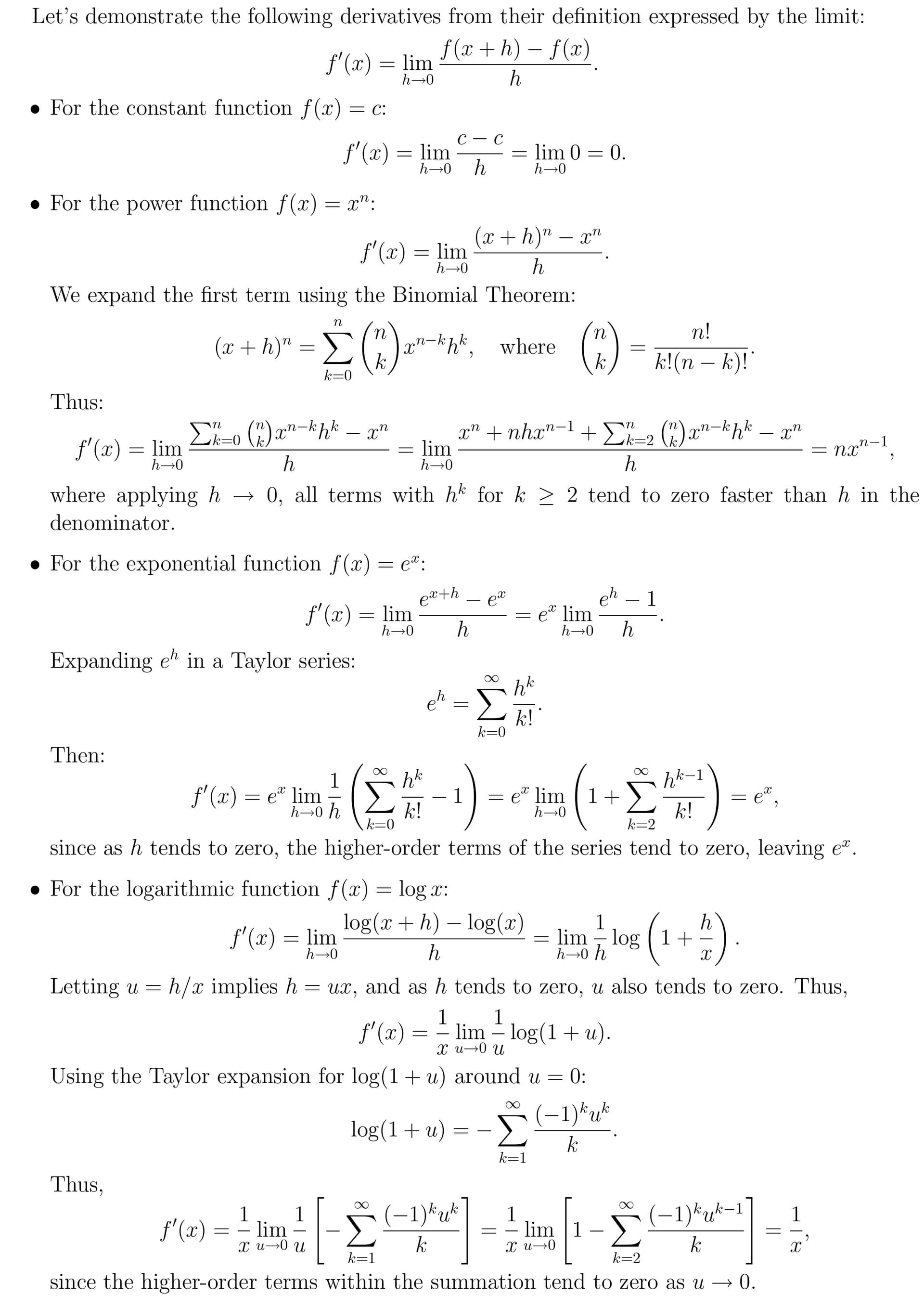
\section*{Problem 1}
For $f(x) = c$ where $c$ is a constant, we have
$$
\lim_{h \to 0} \frac{f(x + h) - f(x)}{h} = \lim_{h \to 0} \frac{c - c}{h} = 0
$$
For $f(x) = x^n$, we have
\begin{equation}
\begin{split}
\frac{df}{dx} &= \lim_{h \to 0} \frac{(x + h)^n - x^n}{h} \\
&= \lim_{h \to 0} \frac{\binom{n}{0}x^nh^0 + \binom{n}{1}x^{n-1}h^1 + \binom{n}{2}x^{n-2}h^2 + \cdots - x^n}{h} \text{ via the binomial expansion} \\
&= \lim_{h \to 0} \binom{n}{1}x^{n-1}h^0 + \binom{n}{2}x^{n-2}h^1 + \cdots \text{ after cancelling $x^n$ and dividing by $h$} \\
&= \boxed{nx^{n-1}} \text{ since all terms with $h$ approach 0} \\
\end{split}
\end{equation}
For $f(x) = e^x$, we have
\begin{equation}
\begin{split}
\frac{df}{dx} &= \lim_{h \to 0} \frac{e^{x + h} - e^x}{h} \\
&= \lim_{h \to 0} \frac{e^xe^h - e^x}{h} \\
&= \lim_{h \to 0} \frac{e^x(e^h - 1)}{h} \\
&= e^x \times \lim_{h \to 0} \frac{e^h - 1}{h} \\
&= e^x \times 1 \text{by L'Hopital's rule} \\
&= \boxed{e^x} \\
\end{split}
\end{equation}
For $f(x) = \log(x)$
\begin{equation}
\begin{split}
\frac{df}{dx} &= \lim_{h \to 0} \frac{\log(x + h) - \log(x)}{h} \\
&= \lim_{h \to 0} \frac{\log\left(\frac{x + h}{x}\right)}{h} \\
&= \lim_{u \to 0} \frac{\log\left(1 + u\right)}{ux} \text{ with } u = \frac{h}{x} \\
&= \frac{1}{x} \lim_{u \to 0} \frac{\log(1 + u)}{u} \\
&= \frac{1}{x} \lim_{u \to 0} \frac{1}{(1 + u)\ln{10}} \text{ by L'Hopital's rule} \\
&= \boxed{\frac{1}{x\ln{10}}} \\
\end{split}
\end{equation}
This proof is a bit circular since it uses the derivative of $\log(x)$ when applying L'Hopital's rule! If you found a better proof, let me know.
\section*{Problem 2}
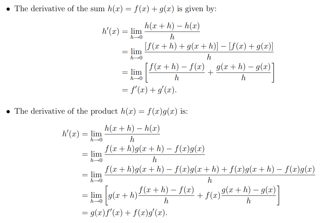
For the product rule:
\begin{equation}
\begin{split}
&\text{Prove } \frac{d}{dx} \left[ f(x)g(x) \right] = f(x)g'(x) + g(x)f'(x) \\
&= \lim_{h \to 0} \frac{f(x+h)g(x+h) - f(x)g(x)}{h} \text{ using the definition of a derivative} \\
&= \lim_{h \to 0} \frac{f(x+h)g(x+h) - f(x+h)g(x) + f(x+h)g(x) - f(x)g(x)}{h} \\
&= \lim_{h \to 0} \frac{f(x+h)\left[g(x+h)-g(x)\right] + g(x)\left[f(x+h)-f(x)\right]}{h} \\
&= f(x+0)\lim_{h \to 0} \frac{g(x+h)-g(x)}{h} + g(x)\lim_{h \to 0} \frac{f(x+h)-f(x)}{h} \\
&= \boxed{f(x)g'(x) + g(x)f'(x)} \\
\end{split}
\end{equation}
For the sum rule:
\begin{equation}
\begin{split}
&\text{Prove } \frac{d}{dx} \left[ f(x)+g(x) \right] = f'(x) + g'(x) \\
&= \lim_{h \to 0} \frac{[f(x+h)+g(x+h)] - [f(x)+g(x)]}{h} \\
&= \lim_{h \to 0} \frac{f(x+h) - f(x)}{h} + \lim_{h \to 0} \frac{g(x+h) - g(x)}{h} \\
&= \boxed{f'(x) + g'(x)} \\
\end{split}
\end{equation}
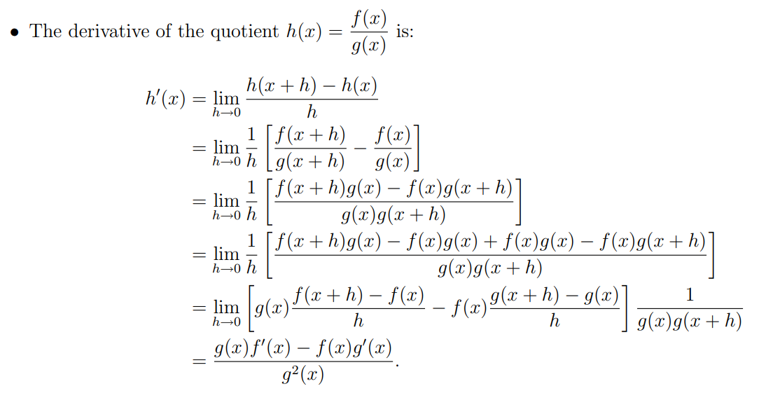
For the quotient rule:
\begin{equation}
\begin{split}
&\text{Prove } \frac{d}{dx} \left( \frac{f(x)}{g(x)} \right) = \frac{g(x)f'(x) - f(x)g'(x)}{g^2(x)} \\
&= \lim_{h \to 0} \frac{\frac{f(x+h)}{g(x+h)} - \frac{f(x)}{g(x)}}{h} \\
&= \lim_{h \to 0} \frac{f(x+h)g(x) - f(x)g(x+h)}{hg(x)g(x+h)} \\
&= \lim_{h \to 0} \frac{f(x+h)g(x)-f(x)g(x)+f(x)g(x)-f(x)g(x+h)}{hg(x+h)g(x)} \\
&= \lim_{h \to 0} \frac{g(x)[f(x+h)-f(x)] - f(x)[g(x+h)-g(x)]}{hg(x)g(x+h)} \\
&= \boxed{\frac{f'(x)g(x) - f(x)g'(x)}{g(x)^2}} \\
\end{split}
\end{equation}
\section*{Problem 3}
The product rule states $\frac{d}{dx}[f(x)g(x)] = f(x)g'(x) + g(x)f'(x)$. Let $g(x) = c$.
$$
f(x)\frac{d}{dx}c + c\frac{d}{dx}f(x) = f(x)\cdot0 + c\frac{d}{dx}f(x) = \boxed{c\frac{d}{dx}f(x)}
$$
\section*{Problem 4}
\begin{equation}
\begin{split}
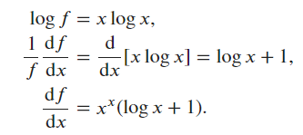
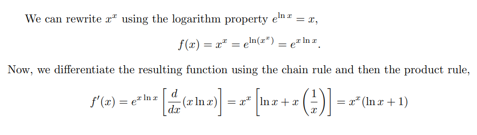
y &= x^x \\
\ln{y} &= \ln{x^x} = x\ln{x} \\
\frac{1}{y}\cdot\frac{dy}{dx} &= \ln{x} + x \cdot \frac{1}{x} \text{ by the product rule} \\
\frac{dy}{dx} &= y(\ln{x} + 1) \\
\frac{dy}{dx} &= x^x(\ln{x} + 1) \\
\end{split}
\end{equation}
\section*{Problem 5}
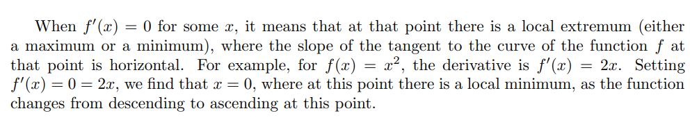
$f(x)$ has a slope of 0 at that point. For instance, $f(x) = x^2$ has a slope of 0 at $x = 0$.
\section*{Problem 6}
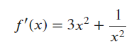
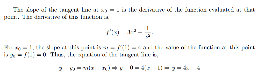
Done using $3x^2 + \frac{1}{x^2}$ to calculate the slope, yielding the final equation $4x-4$.
\section*{Problem 7}
$$
\nabla_x f(x) =
\begin{bmatrix}
6x_1 \\
5e^{x_2} \\
\end{bmatrix}
$$
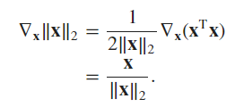
\section*{Problem 8}
\begin{equation}
\begin{split}
f(\mathbf{x}) &= \|\mathbf{x}\|_2 \\
\nabla_{\mathbf{x}} \|\mathbf{x}\|_2 &= \nabla_{\mathbf{x}} (\mathbf{x}^{\top}\mathbf{x})^{1/2} \\
&= 2\mathbf{x} \cdot \frac{1}{2}(\mathbf{x}^{\top}\mathbf{x})^{-1/2} \\
&= \boxed{\frac{\mathbf{x}}{\|\mathbf{x}\|_2}} \\
\end{split}
\end{equation}
At $x=0$, the gradient is undefined.
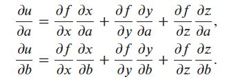
\section*{Problem 9}
$$
\frac{\partial{u}}{\partial{a}} = \frac{\partial{u}}{\partial{x}} \cdot \frac{\partial{x}}{\partial{a}} + \frac{\partial{u}}{\partial{y}} \cdot \frac{\partial{y}}{\partial{a}} + \frac{\partial{u}}{\partial{z}} \cdot \frac{\partial{z}}{\partial{a}}
$$
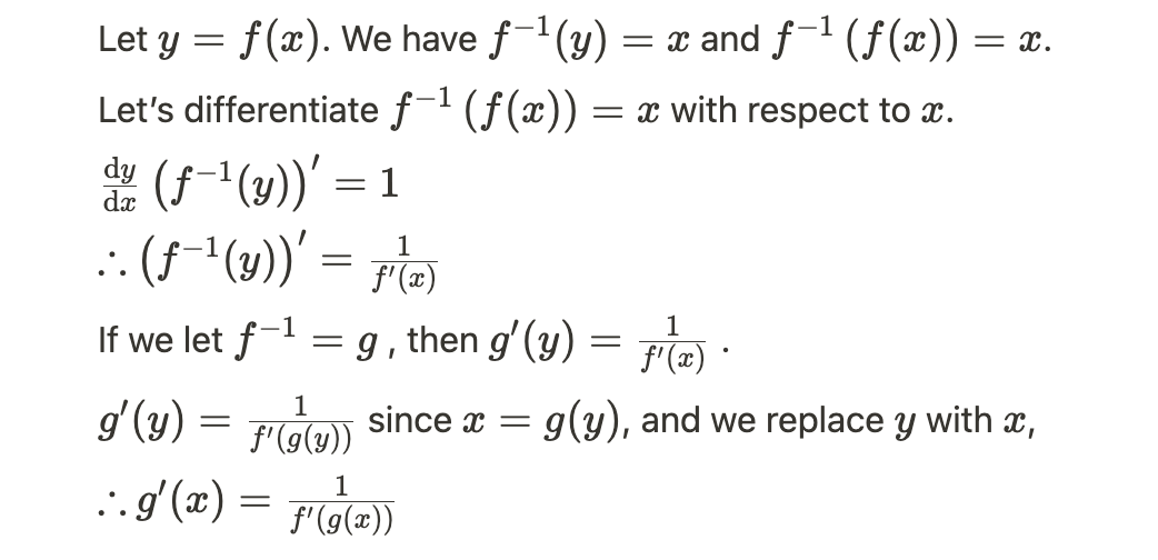
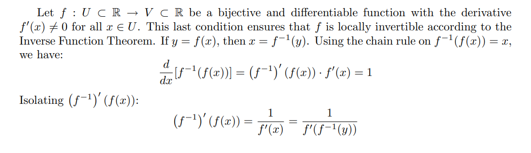
\section*{Problem 10}
\begin{equation}
\begin{split}
y &= f^{-1}(x) \\
x &= f(y) \\
1 &= f'(y) \cdot \frac{dy}{dx} \\
\frac{dy}{dx} &= \frac{1}{f'(y)} \\
\frac{d}{dx}f^{-1}(x) &= \frac{1}{f'(f^{-1}(x))} \\
\end{split}
\end{equation}
\end{document}
Sarah
June 18, 2024, 7:10pm
42
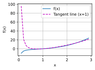
import numpy
import matplotlib.pyplot as plt
# Code omitted to make the graph look nice: `plt.rcParams.update...`
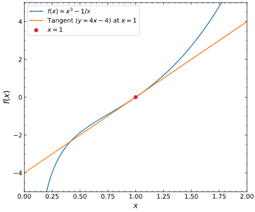
def f(x):
return x ** 3 - 1 / x
def df(x):
return 3 * x ** 2 + 1 / x ** 2
def tangent(x, x_0):
return df(x_0) * (x - x_0) + f(x_0)
x_0 = 1
x = np.arange(0.01, 2, 0.01)
_, ax = plt.subplots()
ax.plot(x, f(x), label="$f(x) = x^3 - 1/x$")
ax.plot(x, tangent(x, x_0), label="Tangent $(y = 4x - 4)$ at $x=1$")
ax.scatter(x_0, tangent(x_0, x_0), zorder=10, color="tab:red", label="$x=1$")
ax.set(xlabel="$x$", ylabel="$f(x)$", xlim=(0, 2), ylim=(-5, 5))
ax.legend();
Source: Inverse function theorem .
2 Likes
your tangent is a line, but your graph shows a curve. Tangent Line is defined as mx+c where m is the slope and c is a constant.
filipv
January 12, 2025, 11:38pm
44
Revisiting this chapter, I remember being confused by the orientation of the gradients listed in section 2.4.3 – as a hint for other readers, I recommend reading the Layout conventions section of the Matrix calculus Wikipedia Article . This textbook’s appendix, specifically section 22.4.7 is also a great resource.
To summarize, there are two popular conventions for vector-vector derivatives:
In the numerator-based layout (sometimes called the Jacobian layout), the derivative has the same number of rows as the numerator’s dimensionality.
In denominator-based layouts (sometimes called the Hessian or gradient layout), the derivative has the same number of rows as the denominator’s dimensionality. This is sometimes notated by using a gradient symbol, as the authors do here. You also sometimes see a transpose symbol in the denominator to hint the reader that the denominator-based layout is being used.
1 Like