I would love some insight into problem 6! I can’t make any headway. Loving the book so far. Thanks
I think this post does a good job at discussing Q6
Here are my opinions about the exs.
ex.1
I close the lot in d2l.Module.
@d2l.add_to_class(d2l.Module)
def training_step(self, batch):
    l = self.loss(self(*batch[:-1]), batch[-1])
    #self.plot('loss', l, train=True)
    return l
@d2l.add_to_class(d2l.Module)
def validation_step(self, batch):
    l = self.loss(self(*batch[:-1]), batch[-1])
    #self.plot('loss', l, train=False)
    return l
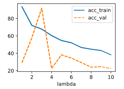
Then I use this code snippet to test lambda from 1 to 10
import numpy as np

data = Data(num_train=100, num_val=100, num_inputs=200, batch_size=20)
trainer = d2l.Trainer(max_epochs=10)
test_lambds=np.arange(1,11,1)
board = d2l.ProgressBoard('lambda')

def accuracy(y_hat, y):
    return (1 - ((y_hat - y).mean() / y.mean()).abs()) * 100

def train_ex1(lambd):
    model = WeightDecay(wd=lambd, lr=0.01)
    model.board.yscale='log'
    trainer.fit(model, data)
    y_hat = model.forward(data.X)
    acc_train = accuracy(y_hat[:data.num_train], data.y[:data.num_train])
    acc_val = accuracy(y_hat[data.num_train:], data.y[data.num_train:])
    return acc_train, acc_val

for item in test_lambds:
    acc_train, acc_val = train_ex1(item)
    board.draw(item, acc_train.to(d2l.cpu()).detach().numpy(), 'acc_train', every_n=1)
    board.draw(item, acc_val.to(d2l.cpu()).detach().numpy(), 'acc_val', every_n=1)
The output of accuracy of different lambda goes like this:
ex.2
I think there may be an analytical solution of lambda if the weights w have already been set after training, and the validation set is fixed, but this procedure gives no credit to any different validation set, so this kind of optimal makes no sense.
I think it doesn’t matter if the lambda is optimal, cause in practice, I can test a set of options and choose one that is good enough to be my lambda.
ex.3
ex.4
ex.5
I think if I can’t narrow gap between training error and generalizing error, there is also a great chance to reach overfitting, so I may use cross validation to make more use on the data I have now.
ex.6
Regularization adds some limit on the parameters of a model before the training, that is somehow like a prior in Bayesian estimation.
1 Like
what is a scratch? please define scratch.
I’m seeing a similar L2 norm of the weights between the example without regularization and the example using ‘weight_decay’ in torch.optim.SGD.
The examples in the book show this as well, whereas the L2 norm of the weights is 10 times smaller for the WeightDecayScratch using a lambda of 3.
Why might we expect this?
I am trying to implement weight decay from scratch, however no matter what I set lambda to, I notice the validation loss is always constant. Is there something wrong with my code?
class Data():
def init(self, num_train, num_val, num_inputs, batch_size):
self.batch_size = batch_size
n = num_train + num_val
self.X = torch.randn(n, num_inputs)
noise = torch.randn(n, 1) * .01
w, b = torch.ones((num_inputs, 1)) * .01, .05
self.y = torch.matmul(self.X, w) + b + noise
self.num_train = num_traindef get_trainloader(self): tensorData = TensorDataset(self.X[:self.num_train], self.y[:self.num_train]) return DataLoader(tensorData, batch_size=self.batch_size, shuffle=True) def get_testloader(self): tensorData = TensorDataset(self.X[self.num_train:], self.y[self.num_train:]) return DataLoader(tensorData, batch_size = self.batch_size, shuffle = False)class WeightDecay():
def init(self, num_inputs, lambd, lr):
self.num_inputs = num_inputs
self.lambd = lambd
self.lr = lr
self.net = nn.LazyLinear(1)
self.net.weight.data.normal_(0, .01)
self.net.bias.data.fill_(0)def forward(self, x): return self.net(x) def loss(self, yhat, y): loss_fun = nn.MSELoss()(yhat, y) L2_reg = self.lambd * ((self.net.weight ** 2).sum() / 2) return loss_fun + L2_reg def configure_optimizer(self): return torch.optim.SGD(self.net.parameters(), self.lr, weight_decay=0)data = Data(num_train=20, num_val=100, num_inputs=200, batch_size=5)
model = WeightDecay(200, lambd=0.1, lr=0.01)
optim = model.configure_optimizer()
train_data = data.get_trainloader()
test_data = data.get_testloader()for i in range(10):
train_loss = 0
for X, y in train_data:
preds = model.forward(X)
lossfun = model.loss(preds, y)
train_loss += lossfun
optim.zero_grad()
lossfun.backward()
optim.step()with torch.no_grad(): test_loss = 0 for X, y in test_data: preds = model.forward(X) lossfun = model.loss(preds, y) test_loss += lossfun print(f"Avg loss for epoch {i + 1} on train is {train_loss / len(train_data)}") print(f"Avg loss for epoch {i + 1} on test is {test_loss / len(test_data)}")
- With greater values of
\lambda, the validation loss goes down far more quickly in early epochs. But no matter how large my setting of\lambda, the validation loss doesn’t seem to go far below 10e-2. For extremely large values, the model fails to converge at all. - The final error continues going down for values of
\lambdawell into the range of 10-50! But in practice, I’m not sure you’d want to use a value so extreme - this example is somewhat contrived, and exaggerates the effect of weight decay. Using values this large in practice would hurt the model’s capacity. - Using
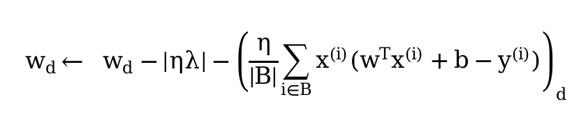
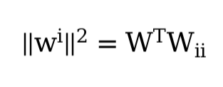
\|\mathbf w\|^2, our update to each parameterw_iis equivalent to\eta \lambda \cdot \mathbf w_i. If we used|\mathbf w|, our updates would not scale relative to the weights, and would be a constant\eta \lambdatimes the sign of w. \| A \|_F^2 = \text{trace}(A^T A). Intuitively, the diagonal entries on the gram matrix of A are where the dot product of each column with itself is located - these are the sums of the squares of each column. When we add them up, all entries are included.- More training data, greater diversity of data (possibly including data augmentation), and other forms of added stochastic noise - for example, the slight stochasticity introduced by batch norm layers tends to regularize the model. This is outside the scope of this chapter, but dropout and early stopping can also help.
- In a basic sense, simpler weights are ‘more likely’, and regularization is a means of increasing our P(w), and therefore the posterior probabilities. Further, we can draw a connection between our prior on the weights and the form of regularization we ought to use - if we assume each weight is drawn from a Gaussian distribution with a mean of zero, minimizing the negative log-likelihood of the weights would suggest penalizing a term proportional to the squared norm of w. Analogously, assuming a Laplacian distribution of the weights, minimizing the negative log-likelihood of the weights suggests penalizing a term proportional to the sum of their absolute values - the L1 norm!
- Review the relationship between training error and generalization error. In addition to weight decay, increased training, and the use of a model of suitable complexity, what other ways might help us deal with overfitting?
Apart from data augmentation, regularization, and choosing a model with suitable complexity, for deep learning methods, we can consider using dropout (to avoid co-adaption of features), early stopping, and parameter sharing (to reduce the number of parameters, such as in CNN). For tree-based methods, we can consider ensemble models. For example, a single decision tree is prone to overfitting, but by creating a random forest, we can reduce variance and counter overfitting.
- In Bayesian statistics we use the product of prior and likelihood to arrive at a posterior via . How can you identify with regularization?
L1 regularization corresponds to a Laplace prior, while L2 regularization corresponds to a Gaussian prior.
Emmmm I feel this is a really bad example of weight decay here.
First, we know that the ground true weight should have give an $\ell_2$ norm as $0.01^2\times 200 /2 =0.01$, so the result with weight decay on actually failed to get a good approximation of the weight value.
Also from the loss aspect. Indeed with weight decay on we see the validation loss is decreasing during training. But the problem is that it’s always even larger than the constant validation loss without weight decay. (The contribution of the penalty is negligible as we know it’s about 0.001, while the full validation loss is larger than 0.01)
This can also be explained when we consider the motion of the weight vector in its 200-dimensional space. The 20 vectors of training data span a subspace of 20 dimension. The problem of the persisted validation loss here is that, our gradient of loss is always constrained in that subspace. Thus the weight vector can only move in such way during training. Since we initialize the weight vector with a 200-dimensional Gaussian with $\sigma=0.01$, it’s much closer to 0 than the ground true weight vector. Then after training the weight vector arrives near the projection of the ground true weight vector.
The problem arises here. We are projecting out 180 dimensions of a 200-dimensional vector, so most of its length is lost, which gives rise to the persisted validation loss without weight decay. But adding weight decay can’t save us from these. Since the initial weight vector is around 0, the gradient from the penalty loss is still constrained inside the 20-dimensional subspace. And the penalty only pulls the weight vector away from the projection, which makes things only worse in the end.
Of course, adding a penalty is expected to make things worse in the end. But the problem here is that the specific initialization setting happens to give a relative good result even without penalty.
To see the power of weight decay, maybe we should change the initialization of the model. For example, changing the sigma of WeightDecayScratch object from the default 0.01 to 1, you will see the result from train_scratch(0) becomes significantly worse, while the result from train_scratch(3) is still similar to the one from previous initialization.