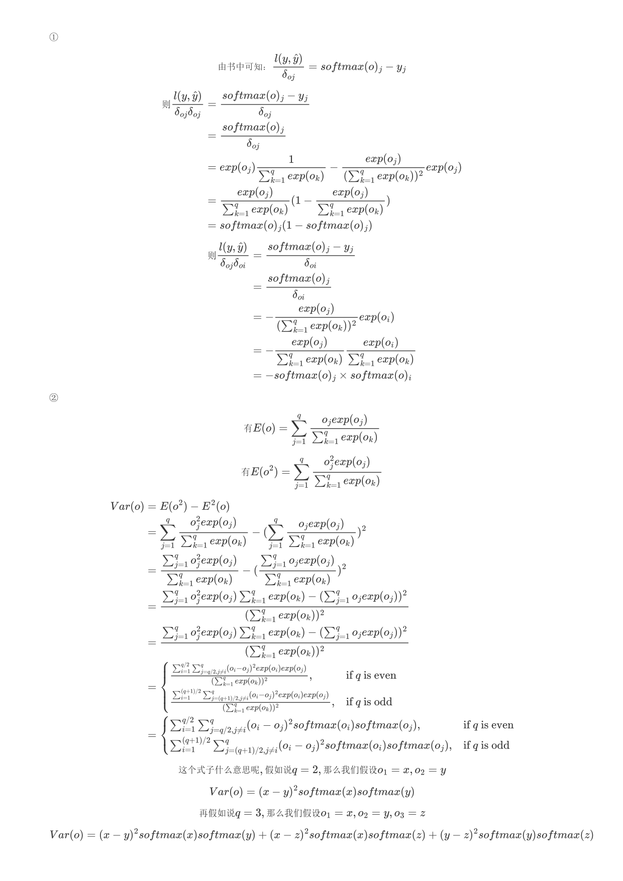
I have a question regarding Excercise 1 of this section of the book. I won’t include details of my calculations in order to keep this as simple as possible. Sorry for my amateurism, but I couldn’t render equations in this box, so I decided to upload them as images. However, because I’m a “new user” I can’t upload more than one image per comment, so I’m posting the rest of this comment as a single image file.
Hey @washiloo, thanks for detailed explanation. Your calculation is almost correct! The reason we are not considering i not equal to j is: you will need to calculate the second order gradient, only when you can explain o_i in some formula by o_j, or it will be zero. There blog here may also help!
Thank you for your reply, @goldpiggy ! However, I don’t understand what do you mean by “only when you can explain o_i in some formula by o_j, or it will be zero”. We are not computing the derivative of o_i with respect to o_j, but the derivative of dl/do_i (wich is a function of all o_i’s) with respect to o_j, and this derivative won’t, in general, be equal to zero. Here, d means “partial derivative” and l is the loss function, but I couldn’t render them properly.
In my early post, I wrote the analytical expression of these second-order derivatives, and you can see that they are zero only when the softmax function is equal to zero for either o_i or o_j, which clearly cannot happen due to the definition of the softmax function.
NOTE: I missed the index 2 for the second-order derivative of the loss function in my early post, sorry.
Hey @washiloo, first be aware that o_j and o_i are independent observations. i.e., o_i cannot be explained by a function of o_j. If there are independent, the derivatives will be zero. Does this helps?
I think we are talking about different things here. You are talking about the derivatives of o_i w.r.t o_j or the other way around (which are all zero because, as you mention, they are not a function of each other), and I’m talking about the derivatives of the loss function, which depends on all variables o_k (with k = 1,2...,q, because we are assuming that the dimension of 𝐨 is q). We both agree that the gradient of the loss function exists, and this gradient is a q-dimensional vector whose elements are the first-order partial derivatives of the loss function w.r.t. each of the independent variables o_k. Now, each of these derivatives is also a function of all variables o_k, and therefore can be differentiated again to obtain the second-order derivatives, as I explained in my first post. But this is not a problem at all… I understand how to compute these derivatives and I also managed to write a script that computes the Hessian matrix using torch.autograd.grad.
My question is related to Exercise 1 of this section of the book:
“Compute the variance of the distribution given by softmax(𝐨) and show that it matches the second derivative of the loss function.”
As I mentioned before, it is not clear to me what do you mean here by “the second derivative” of the loss function. This “second derivative” should be a real number, because the varianceV of the distribution is a real number, and we are trying to show that these quantities are equal. But there are q^2 second-order partial derivatives, so what are we supposed to compare with the variance of the distribution? One of these derivatives? Some function of them?
Does anyone have any idea about Q2? I don’t see the problem about setting the binary code to (1,0,0) (0,1,0) and (0,0,1) on a (1/3, 1/3, 1/3) classification problem. Please reply me if you have any thought on this. Thanks!
I got the same result as you.I also don’t understand why some discussions assume that the second-order partial derivative equals to variance of softmax when i=j.
Sorry guys. here are my wrong answers. I kind of have the feeling that most of this is wrong looking at discussion here. but just putting it here for a sense of completion. But here is my contribution anyway.
Exercises
We can explore the connection between exponential families and the softmax in some more
depth.
1. Compute the second derivative of the cross-entropy loss l(y, yˆ) for the softmax.

* after applying quotient rule for cross entropy loss the anaswer comes out to be zero.apparentlythis is wrong.

2. Compute the variance of the distribution given by softmax(o) and show that it matches
the second derivative computed above.
* Its close to zero through experiments too. but why should this happen? is second derivative essentially same as variance?

Assume that we have three classes which occur with equal probability, i.e., the probability
vector is 1/3
1. What is the problem if we try to design a binary code for it?

* We would need at least 2 bits, and 00,01, 10 would be used but not 11. ?

2. Can you design a better code? Hint: what happens if we try to encode two independent
observations? What if we encode n observations jointly?
* we can do it through one hot encoding where the size of array would be the number of observations n
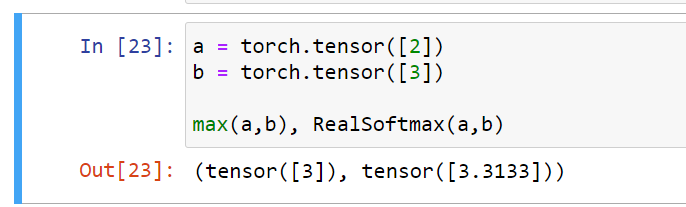
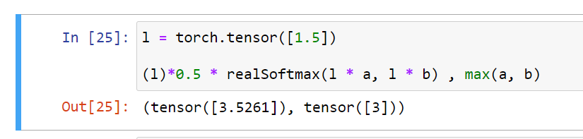
Softmax is a misnomer for the mapping introduced above (but everyone in deep learning
uses it). The real softmax is defined as RealSoftMax(a, b) = log(exp(a) + exp(b)).
1. Prove that RealSoftMax(a, b) > max(a, b).

* verified though not proved
There is a type in the sentence: “Then we can choose the class with the largest output value as our prediction…” it should be y hat at in the argmax rather than y
I’ve got the same result for the second derivative of the loss but I don’t know how to compute the variance or how it relates with the second derivative.
Did you make any progress ?
I am unsure what this question is trying to get at:
Assume that we have three classes which occur with equal probability, i.e., the probability vector is (1/3,1/3,1/3).
What is the problem if we try to design a binary code for it?
Can you design a better code? Hint: what happens if we try to encode two independent observations? What if we encode n observations jointly?
My guess is simply that binary encoding doesn’t work when you have more than 2 categories, and one hot encoding with possibilities (1,0,0), (0,1,0) and (0,0,1) works better.
However, this doesn’t seem to address the specific probability or the hint given, so I think my guess is too simplistic.