Linear Regression

[randomtheorist]

@cclj

To tackle this problem, the learning rate scheduler might help. We manually shrink the learning rate to control the converging process

I think one way to circumvent this is to use the square loss function when the error is small (near stationary point) and use absolute error otherwise. This loss function is known as the Huber Loss function
Info on Huber loss

[randomtheorist]

@pumuckl

I don’t know what is done in this case, but I could imagine that increasing the batch size when the optimization comes closer to a stationary point could be useful, or reduction of the learning rate over time, but this would be certainly a parameter to tune

I think one way to circumvent this is to use the square loss function when the error is small (near stationary point) and use absolute error otherwise. This loss function is known as the Huber Loss function
Info on Huber loss

[rrrrp]

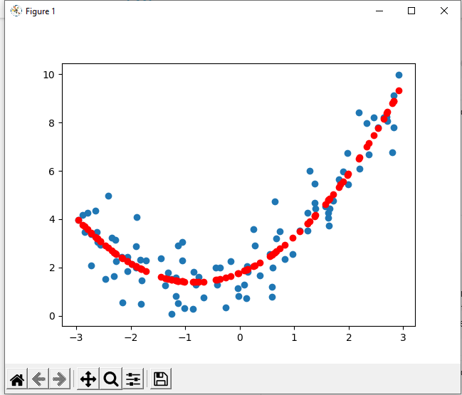
Wanted to point out that this chapter is missing a fairly important point. Although linear regression is often used on linear data, it can also be used on exponential data. With Gradient Descent on Mean Squared Error - the derivative of MSE is always linear with respect to the weights. Although often labeled “polynomial regression” - it is essentially linear regression under the hood.

[rrrrp]

Quick note regarding incorrect usage of the dimension terminology:

[Egor]

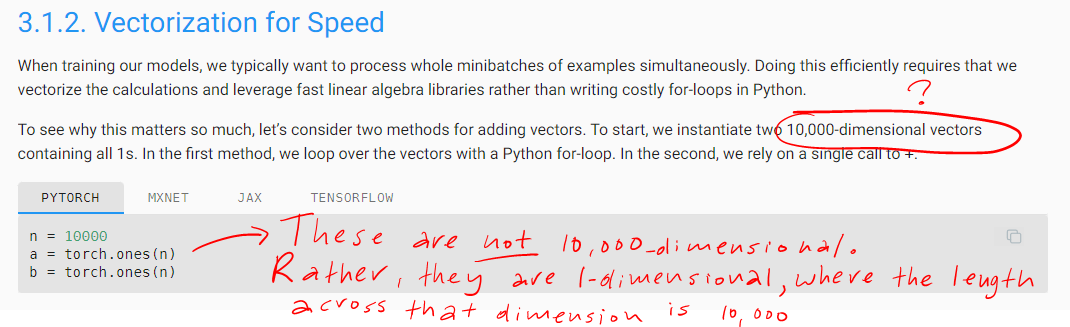
In Chapter 2.3 the authors mention that they use “dimensionality” to refer to the number of elements along an axis: “Oftentimes, the word “dimension” gets overloaded to mean both the number of axes and the length along a particular axis. To avoid this confusion, we use order to refer to the number of axes and dimensionality exclusively to refer to the number of components.”

Talking about the polynomial regression, what do you mean by linear regression under the hood? Linear regression is a special case of polynomial regression but as far as I know they are fairly different.

[emmanuelfv]

Hi, this is indeed correct, here the usage is for vectors, were can be assumed that its space belongs to R^(1*n). A differetent case would be if they mention it as 10,000-dimentional Matrix. In that case there may be an uncertainity about how to allocate dimentions over the matrix.

[filipv]

A note for other readers - this chapter alludes to a connection between MLE over common probability distributions and common loss functions used in ML. Investigate this! Start by finding the negative-log likelihood function of a Bernoulli distribution.

My solutions:

1. Analytically, the optimal value of b is \frac{1}{n} \sum_{i=1}^n x_i, or the mean of the x_i. If we assume the x_i are sample from a normal distribution, the maximum likelihood estimate of \mu is precisely the same sample mean. If we change the loss to \sum_i |x_i - b|, the optimal solution for b is the median of the x_i. I’m not sure how to express this analytically, but visualize the gradient - when b is less than all the x_i, the subgradient wrt b is -1 for each term, making the net subgradient -n. Each time b “passes by” one of the x_i, the gradient increases by 2. The gradient is zero when the same number of terms are to the left and to the right of b - precisely when b is the median!
2. This is trivially true, as a linear combination of the components of \mathbf x are equivalent to \mathbf x^\top \mathbf w, and 1 times some linear weight w can always match an arbitrary scalar b.
3. Naively, why not append {1}, the features of x, and the flatted matrix x*x^T, using the same single-layer architecture as the linear regression case? I get the sense that this question may be asking for something more clever, but it’s very general.
4. If X^\top X is not full rank, you cannot take its inverse - moreover, it means that the column space of X is a subspace. Unless \mathbf y happens to be in that subspace, there’s no set of weights you could learn to express y exactly. Adding a small amount of Gaussian noise to all entries of X would address this - it would “knock coplanar vectors off” their shared planes. The expected value of X^\top X with an added Gaussian noise matrix N is equal to X^\top X + \text E[N^\top N], but there may be a way to simplify further. If X^\top X is not full rank stochastic gradient descent wouldn’t lead towards a single minima, but anywhere along the line (or plane, etc) of solutions. This can be addressed by adding a weight decay term to the loss.
5. The negative log likelihood is -\log P(y|x) = n\log{2} + \sum_{i=1}^n |y^{(i)} - \mathbf w^\top x^{(i)} - b|, for which there’s no closed-form solution as far as I can tell, as this | \cdot | form is not differentiable at zero. When performing gradient descent, one could use \frac{\partial}{\partial \mathbf w} of \mathbf x_i when \epsilon \gt 0 and -\mathbf x_i when \epsilon \lt 0, but this might cause the gradients to “bounce around” as the model converges on the stationary point. You might be able to fix this with a decaying learning rate schedule (such that the update size grows progressively smaller as the model converges on the stationary point).
6. The composition of two linear layers is itself a linear layer - you’d have to place some kind of nonlinearity between the two layers to increase the network’s representational capacity.
7. A gaussian model allows for negative predictions which don’t apply to money, and prices tend to move in a multiplicative fashion (the price going up by 10% is more relevant than a specific dollar amount). Using log(price) addresses these concerns, as log is strictly positive and captures changes in ratios (multiplicative change). Penny stocks could cause issues as they’re close to zero (meaning log(price) approaches negative infinity), and are small enough that the fact that money is technically discrete (in cents) could begin to cause issues.
8. A Gaussian additive noise model doesn’t work well since apples are discrete units, but a Gaussian distribution models continuous phenomena. The proof for the second part is interesting - as a hint for other readers, it involves the Taylor series of e^x. As for the loss function, assuming this just means taking the negative log-likelihood and dropping terms which don’t contain the parameters, L_\lambda = \lambda - k\log{\lambda}. For 8.4, let x = \log{\lambda} - the result obtained is -\log P(k | \lambda = x) = e^x - kx.

[rdong8]

For Q8.3 do we still model the problem as y = w^T x + b + epsilon where epsilon is a Poisson random variable? Do we have to restrict w to be a vector of integers?