hi @goldpiggy may i know how to evaluate analytical solution
Can u help by solving the first qn
thanks
Hi.
In chapter 3.1.1.3 we got the analytical solution by this formula:
w∗=(X⊤X)−1X⊤y
by that, we have a hidden assumption that X⊤X is reversible matrix.
how can we assume that?
thanx a lot.
1 Like
If anyone knows the answer of Q3 of exercise, I will be more than happy if you comment me 
My current answer:
- neg-likelihood: sum(on i from 1 to n) of |y_i - x_i’w|
- I have no idea how to obtain the gradient of sum of absolute values.
- Since the target function is the sum of absolute values of linear combinations of w, the gradient of w, no matter how complicated it can be, must be piecewise constant. Which means, the gradient can never converge to 0, which means there is no STOP of updating w.
How to fix: I have no good idea. Maybe we have to make the learning rate converge to 0 during learning.
1 Like
when we regard x as random variable and w, b as known parameters, then that’s the density function. We all know that.
But then the x are sampled and known, but parameters w, b are unknown, on this condition the same formula becomes the “likelihood function”. So we don’t derive likelihood, we just rename the density as likelihood(However the situation is different).
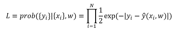
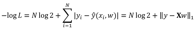
This is my answers for Q3.
- Assume that y=Xw+b+ϵ,p(ϵ)=1/2e^(−|ϵ|)=1/2e^(−|y−y^|) . So , P(y|x)=1/2e^(−|y−y^|) .
Negative log-likelihood: LL(y|x)=−log(P(y|x))=−log(∏p(y(i)|x(i)))=∑log2+|y(i)−y^(i)|=∑log2+|y(i)−X(i)w−b| - ∇{w} LL(y|x)=X.T*(Xw−y/|Xw−y|)=0 . From the equation, we get that: (1) : w=(X.T X)^−1 X.T y and (2) w≠X^−1 y
About Q3.3, I am confused about loss function.
First, please confirm my opinion that determining loss function might affect to the prior assumption of Linear regression model, specially noise distribution and vice versa. In the book, there is a sentence “It follows that minimizing the mean squared error(MSE) is equivalent to maximum likelihood estimation of a linear model under the assumption of additive Gaussian noise.” So what if linear model do not follow Gaussian noise but other noises, can we use MSE (y-y_hat)^2 for loss function again? Or use principle of maximum likelihood( which lead to another loss function ,i.e |y-y_hat|).
Second, how can we determine loss function if we don’t know about noise distribution in practical data? I think we may use some normality test to test the normality of data, but what if the data do not follow Gaussian distribution but p(ϵ) = 1/2*e^(−|ϵ|) for example?
Thanks a lot
1 Like
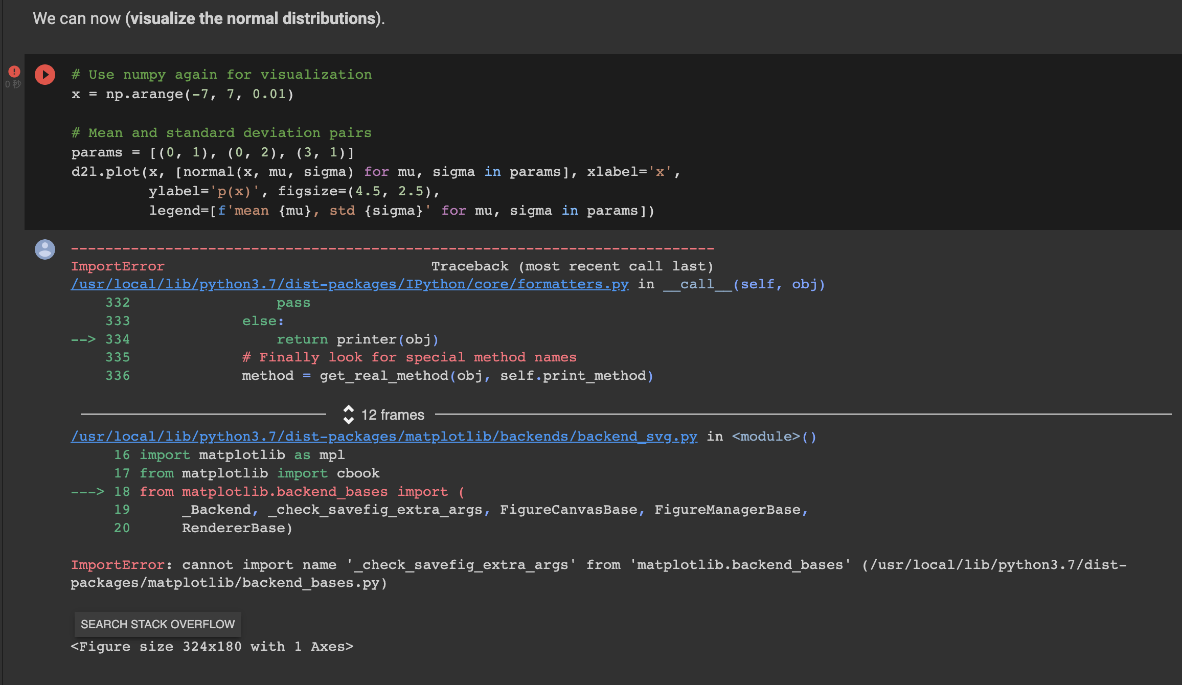
“3.1.2 Vectorization for Speed
When training our models, we typically want to process whole minibatches of examples simulta-
neously.”
From my understanding, the above statement should have “minibatch” rather than “minibatches”…
Thank you
Nisar
The section 3.1.3 is a bit difficult to understand. I have 2 questions:
i) In formula 3.1.13, Why P(y|x) equals to P(ϵ) ?
ii) And does ϵ equals to y minus y_cap ?
Thanks a lot!
No, “minibatches” is fine here. Compare this to:
She likes gummy bears so much, that she typically eats whole packets of them at one sitting.
Here “packets” is the right word, not “packet”.
The following sentence is not easy to parse:
Certainly, the high-level idea that many such units could be cobbled together with the right connectivity and right learning algorithm, to produce far more interesting and complex behavior than any one neuron alone could express owes to our study of real biological neural systems.
Adding some parentheses seems to make it clearer:
Certainly, the high-level idea that many such units could be cobbled together with the right connectivity and right learning algorithm—to produce far more interesting and complex behavior than any one neuron alone could express—owes to our study of real biological neural systems.
Or:
Certainly, the high-level idea that many such units could be cobbled together with the right connectivity and right learning algorithm (to produce far more interesting and complex behavior than any one neuron alone could express) owes to our study of real biological neural systems.
Here are my wrong answers.
- Assume that we have some data
∑x1, . . . , xn ∈ R. Our goal is to find a constant b such that (xi − b)2 is minimized.
1. Find a analytic solution for the optimal value of b.

* solving for xi = b

2. How does this problem and its solution relate to the normal distribution?

* if xi=b then normal equation becomes 1/rootof(2 * pi * sigma^2) * exp(0)  == 1/rootof(2 * pi * sigma^2)
- Derive the analytic solution to the optimization problem for linear regression with squared
error. To keep things simple, you can omit the bias b from the problem (we can do this in
principled fashion by adding one column to X consisting of all ones).
1. Write out the optimization problem in matrix and vector notation (treat all the data as
a single matrix, and all the target values as a single vector).
* X = [[2,3],[4,5]] , y = [0,1]
2. Compute the gradient of the loss with respect to w.
* Not really what was asked but -

3. Find the analytic solution by setting the gradient equal to zero and solving the matrix
equation.
* The questions subpoint tell you how to do it step wise. we have to minimize || y- Xw ||^2 so differentiating w.r.t w and putting it to zero, we have 2X(y-Xw) = 0, which means = Xy = X.Xw w = (X.X)^-1* Xy.

4. When might this be better than using stochastic gradient descent? When might this
method break?
* This method would be good for small datasets, but on larger datasets the cost of storing the entire data in memory and multiplication may be prohibhitive.
- Assume that the noise model governing the additive noise ϵ is the exponential distribution.
That is, p(ϵ) = 1/2 * exp(−|ϵ|).
1. Write out the negative log-likelihood of the data under the model − log P(y | X).

* 1/2 * exp(-|1/root(2 * pi * sigma ^ 2) * exp(-1/(2 * sigma **2) * (x- mu) **2)|) ? what is exponential distribution formula?

2. Can you find a closed form solution?

hmm not quite.

3. Suggest a stochastic gradient descent algorithm to solve this problem. What could possibly go wrong (hint: what happens near the stationary point as we keep on updating the parameters)? Can you fix this?

Not really know whats going on here.In linear regression the epsilon is called error, noise, or disturbance. In classical linear regression context, say, it is this error that has distribution, for instance, N(0, sigma^2). Theoretically, this normality assumption is critical in applying linear regression. Not only for obtaining maximum likelihood estimator for each of parameters, but also for making inference. On the other hand, residuals can be obtained once you have sample. In linear regression theory, the error and the residual have different variances. However, in practice, we can use residual as proxy for the error.
Thank you @gphilip
From deeplearningbook.org I understood why it should be minibatches:
from section 8.1.3:
“Many optimization problems in machine learning decompose over examples well enough that we can compute entire separate updates over different examples in parallel. In other words, we can compute the update that minimizes J(X) for one minibatch of examples X at the same time that we compute the update for several other minibatches. Such asynchronous parallel distributed approaches are discussed further in section 12.1.3.”
Oh well, I read your original question as one about grammar, not about how the training process works!
Hi Halu,
You’re right that the solution (3.1.8) is only correct if (X⊤X) is invertible. In the case where (X⊤X) is not invertible (which happens when the columns of X are dependent), it turns out that the set of weights w*,
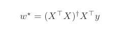
minimizes the loss function (3.1.6). Here, X^+ is the pseudoinverse of X. In essence, every matrix has a pseudoinverse, and the pseudoinverse of an invertible matrix is equivalent to its inverse. You may refer to
for more information about pseudoinverse, its properties and a proof of the above equation.
Numerically, computing the pseudoinverse of an n x n matrix takes O(n^3), which is similar to computing inverse.
I believe that the authors did not discuss the more general case, because of its technicalities, but they omitted to make the implicit assumption that you pointed out.
Excercise 3 (Median regression?)
This was more interesting than I thought initially.
With the likelihood
and the prediction
![]()
the negative log-likelihood should be
 .
.
This is kind of a closed-form solution that should be easily vectorizable.
I could not find a closed-form analytical solution to the gradient in respect to the weights to solve ![]() though. The farthest I got was
though. The farthest I got was
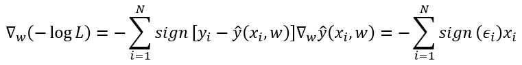
where
The gradient is therefore not a smooth function and has jumps where the residual changes its sign (i.e. where the prediction exactly hits a data point to be predicted).
The problem with stochastic gradient descent (and probably to some extent also to the case where all the data is used) could be that near the stationary point the gradient would jump by flipping the sign of a single vector
I don’t know what is done in this case, but I could imagine that increasing the batch size when the optimization comes closer to a stationary point could be useful, or reduction of the learning rate over time, but this would be certainly a parameter to tune.
I would try also to average the gradient between minibatches, e.g. so that the gradient used to update the parameters consists of some small constant ![]() times the gradient of the current batch plus
times the gradient of the current batch plus ![]() times the gradient of the previous batch. Unfortunately, this would make parallelization over batches difficult.
times the gradient of the previous batch. Unfortunately, this would make parallelization over batches difficult.
Maybe there’s also a way to smooth the jumps?
1 Like
Its the issue with the matplotlib version. Try updating it
I still have some problem in ex.5_C, ex.7_A, can anybody help me with them?
My opinions about the exercises:
ex.1
A.
   ∂ ∑(𝑥𝑖−𝑏)^2 = 0
-> ∂(∑𝑥𝑖^2 + nb^2 - 2b∑𝑥𝑖) = 0
-> 2nb - 2∑𝑥𝑖 = 0
-> b = (∑𝑥𝑖)/n
B. Assume that y = b + 𝜖 where the noise 𝜖 is normally distributed, if we want to maximize the likelihood of the entire dataset, then we will minimize ∑(𝑥𝑖−𝑏)^2.
C.cannot get an analytical solution because absolution doesn’t have a derivative.
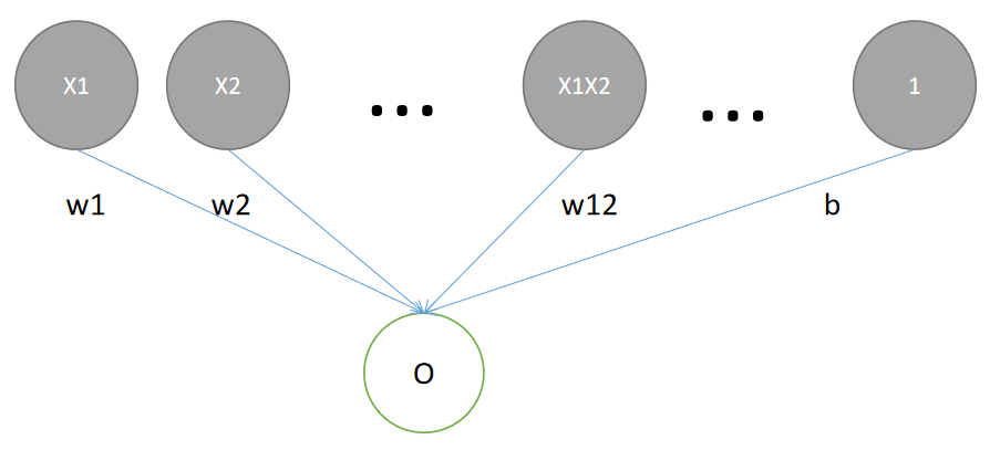
ex.2
theory: (xT, 1) * (w; b) = xTw + b
code:
import torch
def ex2_affine(w, x, b):
    result_by_affine = torch.mm(x.T,w)+b
    print("result_by_affine:\n",result_by_affine)
def ex2_linear(w, x, b):
    b_in_row = torch.ones(x.shape[1]).unsqueeze(0)
    x_and_one = torch.cat((x,b_in_row),0)
    w_and_b = torch.cat((w,torch.tensor([b]).unsqueeze(0)),0)

    result_by_linear = torch.mm(x_and_one.T, w_and_b)
    print("result_by_linear:\n",result_by_linear)

w = torch.tensor([1.,2.]).unsqueeze(1)
x = torch.randn([2,3])
b = 3.
ex2_affine(w,x,b)
ex2_linear(w,x,b)
result_by_affine:
tensor([[1.4326],
[3.2007],
[2.7533]])
result_by_linear:
tensor([[1.4326],
[3.2007],
[2.7533]])
ex.3
ex.4
A. There will be more than one (actually infinite) optimal solution for (w,b).
B. I think we can drop out the dependent dimension(s) from each example, which means we will reduce the number of dimensions of both x and w.
But if we add a coordinate-wise independent Gaussian noise to each dependent dimension(is that what “small amout” means, I’m not so sure about the statement in this question), so we can make the design matrix to have full rank.
C. Given that each Gaussian noise 𝜖∼N(𝜇,𝜎^2) is independent from each other, the element at ith row and j col of design matrix X.TX will be:
XiXj
= ∑[for all d] XidXjd
= ∑[for all originally indenpentdent dimension d] Xid * Xjd
+∑[for all idenpentdent dimension d] Xid * Xjd + 𝜖d ^ 2 + 𝜖d *(Xid + Xjd)
and the expectation of it will be(Ed and 𝜇d is the expectation of dth diemention and the Gaussian noise added on it)
∑(for all dimension d) Ed ^ 2
+∑(for all idenpentdent dimension d) 𝜇d ^ 2
+∑(for all idenpentdent dimension d) 2 * 𝜇d * Ed
D. If we compute the partial derivative of one dependent dimension u, which is depent on v, say, u = f(v), then the result will be like ∂ul + ∂vl * ∂uf’, the same thing happens when we compute on dimension v.
ex.5
A. −log𝑃(𝐲∣𝐗) = ∑ |𝑦−𝐰⊤𝐱−𝑏|
B. There is no close-formed solution cause the absolute.
C. ???
ex.6
As each input of the second layer is like w1x1 + w2x2 +…, some of them may become very large while others become very small, and that may break the balance among the weights of the second layer.
ex.7
A. The Gaussian noise varies from negative infinite to positive infinite, so it’s possible that the price will take a negative value, that is not appropriate.
But for the existing fluctuation, maybe the squared Gaussian noise is useful.(??? I’m not so sure.)
B. If we use logarithm of the price, the price will be limited to be positive.
C. If the price takes a very penny value, the logarithm of it will go to a very large negative number, that may cause overflow. As the price for a house is always not so penny, we may need to drop the peenystocks in our dataset.
ex.8
A. As the Gaussian noise is a continuous value while the number of apples is a discrete value, we cannot use Gaussian noise without any preprocessing.
B.
I searched on the internet an found this, note that the core idea is using Taylor’s formula for e^x.
C.
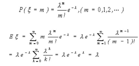
Assume that each example is fetched independently, so the maximum likelihood for the X is like:
argmax[𝜆] P(X)
->armax[𝜆] ∏(𝜆^x * 𝑒^(−𝜆)/x!
→ argmax[𝜆] log(∏(𝜆^x * 𝑒^(−𝜆)/x!)
→ argmin[𝜆] -∑log(𝜆^x * 𝑒^(−𝜆)/x!)
→ argmin[𝜆] -∑(x * log𝜆 - 𝜆 - log(x!))
→ argmin[𝜆] -log𝜆∑x + n𝜆
So the loss function is (-log𝜆∑x + n𝜆), where n is the number of examples.
D. According to C, the loss function for log𝜆(denoted by L) will be
(-L∑x + n * e^L)
2 Likes
ex1:
a. The analytical solution is: b = x_(bar), x_bar is the sample mean.
b. The problem is a sum of residual problem, and the solution is the maximum likelihood estimator of b. By a statistical theorem, the MLE follows a normal distribution with the mean being the MLE and variance being the inverse of the observed fisher information.
c. the analytical solution is b = x_bar. The key is to transform the absolute value into square root of the square of x_i - b.
Hi,
Just to clarify terminology here, on 3.1.1.4 where it says:
“The most naive application of gradient descent consists of taking the derivative of the loss function, which is an average of the losses computed on every single example in the dataset”
Would it be a cost function instead of the loss function due to the fact that the loss function is for one example, while the correct terminology for a cost function is the average over every example?
Thank you,
Ethan