Yeah, that’s right. I guess another way to think about it is to imagine that these data are some sensor output. The sensor has a systematic error that adds .1 to all measurements. Without knowing about that systematic error, an ideal model of the data can be perfectly accurate to the sensor but can never overcome the systematic bias to be perfectly accurate to the thing the sensor is measuring.
In this notebook, we’re adding non-systematic error, but the principle is the same: The best any model can recover is the sample statistics because we don’t know the population parameters (well, we do because we defined the true_* variables, but the model doesn’t have access to that). So my thought was that the ANN should be compared to the maximum-likelihood estimator, not the true underlying parameter (which the ML estimator also wouldn’t know).
Anyway, it was just a thought; I don’t want to make a big deal of it because it’s more academic than practical
@Steven_Hearnt
I still feel confused about what you are talking.
In my understanding, linear relationship is just our idea to simplify a relationship, that maybe we get a hint from Newton “F=ma”.
And then we use words like “noise” to present what isn’t no linear.
So if you have distibution having 0.1 mean, that mean we can add this “0.1” to linear relationship. That is b.
Am I right?
Since y_hat is generated by linreg() , its shape will be batch_size * 1 , which is the same as y , then why is y.reshape(y_hat.shape) necessary? I get wrong results after deleting it.
I tested the code in MXNET colab link and removed the reshape method. It worked fine for me, you might be missing something. Also the reshape is done like a sanity check i guess, so that it won’t raise an error.
Yeah, I removed the reshape call and it didn’t make a difference, since y_hat and y are the same shape. I do wonder if the intent is to keep re-using squared_loss in other parts of the book that may not have the same shape, since it is #@save?
for epoch in range(num_epochs):
for X, y in data_iter(batch_size, features, labels):
l = loss(net(X, w, b), y) # Minibatch loss in X and y
# Compute gradient on l with respect to [w, b]
l.sum().backward()
sgd([w, b], lr, batch_size) # Update parameters using their gradient
with torch.no_grad():
train_l = loss(net(features, w, b), labels)
print(f’epoch {epoch + 1}, loss {float(train_l.mean()):f}’)
What does l.sum().backward() do? How does it process?
Because maybe the number of examples cannot be divided by batch size. For e.g, we have 105 examples and batch size was set to 10. That’s why we use
indices[i:min(i+batch_size, num_examples)]
to catch the last batch whose size is less than 10.
tensor_a.sub_(tensor_b) is equivalent to tensor_a = tensor_a - tensor_b
sub_() is an in-place function.
I suggest you to test the function by some simple data to see the result, or you can just google it.
There is no mistake. For the reason why param.grad is divided by batch_size, you can learn the knowledge of the computational graph. You will find the reason in that part.
Q2: Assume that you are Ohm trying to come up with a model between voltage and current. Can you use auto differentiation to learn the parameters of your model?
A2: You could set the feature of the model to be either V for voltage or I for current. Then, you could take measurements of V as a function of I or I as a function of V on a given conductor to obtain a set of measured of feature-label pairs. Then, these pairs could be used to fit a linear regression model through the gradient descent technique. The weights obtained in the process would (approximately) correspond to the resistance of the conductor from which the measurements were taken. However, these model would give poor prediction results for different conductors with varying resistance. A linear regression model should be built for different conductors. (Remember Ohm’s law V = R*I)
Q4: What are the problems you might encounter if you wanted to compute the second derivatives? How would you fix them?
A4: Apparently, there is no straightforward manner to compute second order derivatives of our loss function using MxNet. However, any differential equation of order n can be written as a system of n differential equations of first order. By solving all of these ODEs of first ordre one could arrive to the solution, but I’m not sure how to implement it. Any suggestions?
It computes the gradient of the tensor l.sum() with respect to w and b. Here is the documentation for this method.
The change is in the gradients, which are stored at the “free variables” w and b with respect to which the gradients are computed. You can retrieve these gradients, and see that they indeed change before and after a call to backward(), by inspecting the grad attribute of these variables, like so: w.grad , b.grad .
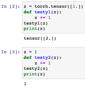
In the function sgd(params, lr, batch_size) this line baffles me:
param -= lr * param.grad / batch_size
How is it possible for this line to update the external scope variable “w”? I did some testing and found the below behavior. Why does the first example update “z” whereas the second does not. Are scope rules different for PyTorch tensors?