https://d2l.ai/chapter_linear-classification/softmax-regression-concise.html
- batch_size num_epochs lr
- It didn’t happen in my training. Why?
I guess that the reason of “the test accuracy decrease again after a while” is that SGD updates too often.
Maybe we can try MBGD.
for more:
Hi @StevenJokes, we talked about the varied optimization algorithms in https://d2l.ai/chapter_optimization/index.html. Hopefully it helps!
I will learn it next time !
when testing the accuracy in concise Softmax regression, it seems that the max of the logits of the each example is used to determine the most probable class rather than the max of exp of logit. since that softmax is implemented in the cross entrophy loss, how did you do softmax in testing

where is it used? cant find it (reply should be at least 20 characters)
Hi,
I have a question about the LogSumExp Trick. In the equation of " Softmax Implementation Revisited" section, we still have this part 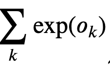 as part of LogSumExp trick. But this is still a exp() calculation of logit. Then how does this method solve of overflow problem? Thank you!
Great question @Philip_C! Since we are optimizing 𝑦̂ to a range of [0,1], we didn’t expect “exp()” to be a super large number. This LogSumExp trick is to deal the overflowed numerator and denominator.
1 Like
Thank you for your reply!
But I still have questions here. ∑𝑘exp(𝑜𝑘) is still calculating the exp() of the logit O, which can still be a large number, thus having the same overflow issue, right?
I want to give a more specific example about why I still don’t understand this trick. For example, let’s assume that we have a logit outcome coming from the model as O = tensor([[-2180.4433, -1915.5579, 1683.3814, 633.9164, -1174.9501, -1144.8761, -1146.4674, -1423.6013, 606.3528, 1519.6882]]), which will become the input of our new LogSumExp Trick loss function.
Now, in our loss function in the tutorial, we have the first part Oj, which do not require exp() calculation. Good. However, we still have the part exp(Ok) in the second part of the new loss function and this part still requires the exp() calculation of every element of the logit outcome O. Then we will still have the overflow issue, e.g. for the last element of O, we will have an overflow error for exp(1519.6882).
This is the part I am still confused. Thank you!
Hi @Philip_C, great question! Logsumexp is a trick for overflow. We usually pick the largest number in the tensor as o_j. i.e., we choose ![]() in
in 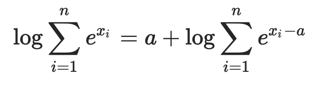 . Please see more details here.
1 Like
Thank you! I got it now. I have to subtract the largest value a from it. I misunderstood it as I thought you don’t have to do that and it was another failed solution.
1 Like
Hi there,
I have copied the code precisely for both this tutorial and the previous one into an IDE (VS Code), and though it runs without errors, it does not produce any visualisations as depicted. It simply completes running silently. Are the graphs only available in a jupyter-like notebook environment?
Exercises
- Try adjusting the hyperparameters, such as the batch size, number of epochs, and learning
rate, to see what the results are.
- changing batch_Size increases time, more epochs trainingaccuracy is more or less constant, learning rate we have to try, changing to 1 loss increases, 0.01 converges slowly.
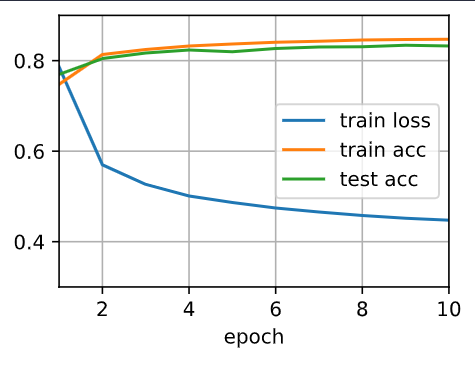
- Increase the number of epochs for training. Why might the test accuracy decrease after a
while? How could we fix this?
- maybe overfitting
They are not available only in jupyter notebooks, however jupyter does have a special way of displaying plots that makes things much easier.
When I use the PyCharm IDE I have to use either scientific mode, save the plots to a file (ie png), or debug the line of code containing “fig.show()” to view my plots. These are the only solutions I have found so far in PyCharm. Hope that helps!
Could you please help me with the following issue: when trying to run d2l.train_ch3 in this notebook, I get the error as in the left side of the attached picture. I realized that the package d2l does not contain the correct train_epoch_ch3 function, so I copied the correct one (from the 3.6 jupyter notebook) into the d2l package file. However, the error persists, as shown in the right side of the picture. Can you please offer some assistance?
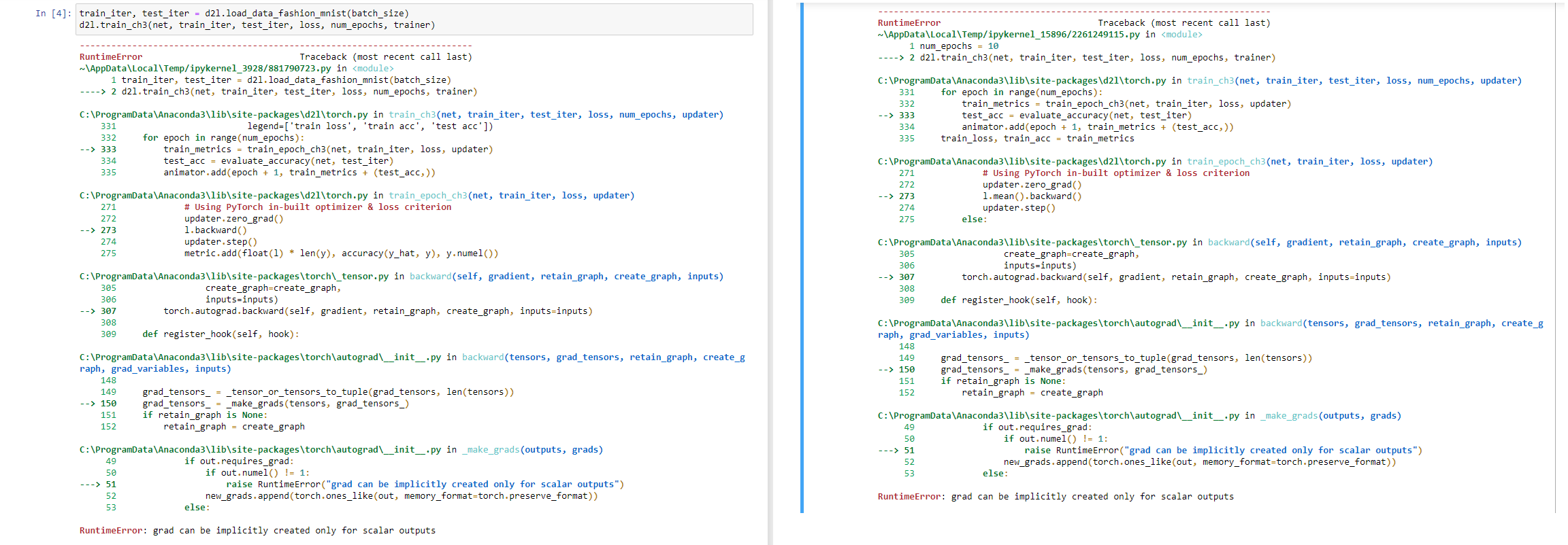
when i saw this error i saw that in the pytorch discusion they indicated that this is most probably due to the loss being a multidementional tensor and that the solution is to “perform some reduction or pass a gradient with the same shape as loss.”
I then just changed the code in the CrossEntrypyLoss function to remove the reduction = ‘none’. The code then ran fine after that and i saw similar results in training to Softmax regression from scratch.
loss = nn.CrossEntropyLoss()
When running in an IDE or from the command line you can display the matplotlib plots by adding “import matplotlib.pyplot as plt” to the imports and then “plt.show()” at the end. This is enough to get the plots displayed when plt.show() is reached (e.g. at the end)
If you want the plots updated after each epoch, then add plt.ion() to put matplotlib into interactive mode, and then plt.pause(0.02) whenever you want the plot updated (for example at the end of each epoch). This allows matplotlib’s GUI loop to run for long enough (0.02s for example) to redraw the plot. At the end, you can say plt.show(block=True) to keep the plot visible if that’s what you want.