Linear Regression Implementation from Scratch

@StevenJokes your understanding of graadients is wrong.

Let me give you a high school example.
Let’s say.
y= wx (Where x is a constant)
The dy/dw = x It doesn’t matter what the value of w is. Gradient is always x.

Get the point?
Similarly when weights are set to zero. gradient is not zero.

If you don’t believe me and you want to print out the gradient value to check:
Then do this small experiment.

X = torch.ones(10,2)
w = torch.zeros((2,1), requires_grad=True)
b = torch.zeros(1, requires_grad=True)
y = torch.matmul(X, w) + b
y.sum().backward()

print(w.grad)
>>>tensor([[10.],
        [10.]])

print(X.sum(dim=0))
>>>tensor([10., 10.])

I just knew that gradient is dy/dw instead of dy/dx. :joy:

We calculate the derivates with respect to weights and not the inputs.
Is this clear now?

Thanks a lot. I got it why I was worry.

Can you close the issue if your doubt is solved? @StevenJokes

You meant my github’s issue?
My issue is about " 2.5.2 does’t have PyTorch’s version."

I have heard that Variable has merge into tensor from zhihu.
Is it right?
If so, 2.5.2 doesn’t need PyTorch’s version.

I have replied to the thread. I think that will answer your questions.
Yes, I meant closing the issue on github if your doubt is solved.

1 Like

Could anyone explain why in the pytorch implementation we have implemented the line param.grad.data.zero_() ?

Why are we setting the gradients of the parameters to 0 after subtracting them from the parameter values? I made my model without this line and my loss kept increasing and reached inf. Also the values of my parameters w, b are large negative values.

# PyTorch accumulates the gradient in default, we need to clear the previous
# values.
x.grad.zero_()

in http://preview.d2l.ai/d2l-en/PR-1080/chapter_preliminaries/autograd.html!

You can use the searching image to find whether a function have mentioned before.

2 Likes

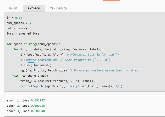
When I run the training code, I got the error:

‘AttributeError: ‘builtin_function_or_method’ object has no attribute ‘backward’’

with l.sum.backward()
How could a loss function we defined by ourselves be autograded ?

I can’t give your answer without the whole code you ran. Please publish your all code you ran.

Thanks for your reply. below is all my code.

%matplotlib inline
from d2l import torch as d2l
import torch
import random
def synthetic_data(w, b, num_examples):
    """ Generate y = Xw + b + noise. """
    X = torch.normal(0, 1, (num_examples, len(w)))
    y = torch.matmul(X, w) + b
    y += torch.normal(0, 0.01, y.shape)
    return X, y.reshape((-1, 1))
​
true_w = torch.tensor([2, -3.4])
true_b = 4.2
features, labels = synthetic_data(true_w, true_b, 1000)
print('features:', features[0], '\nlabel:', labels[0])
features: tensor([ 0.5924, -1.3852]) 
label: tensor([10.1155])
d2l.set_figsize()
# The semicolon is for displaying the plot only
d2l.plt.scatter(d2l.numpy(features[:, 1]), d2l.numpy(labels), 1)
<matplotlib.collections.PathCollection at 0x7f18c1d59750>
def data_iter(batch_size, features, labels):
    num_examples = len(features)
    indices = list(range(num_examples))
    #The examples are read at random, in no particular order
    random.shuffle(indices)
    for i in range(0, num_examples, batch_size):
        batch_indices = torch.tensor(
            indices[i:min(i+batch_size, num_examples)])
        yield features[batch_indices], labels[batch_indices]
batch_size = 10
​
for X, y in data_iter(batch_size, features, labels):
    print(X, '\n', y)
    break
tensor([[-0.9675,  0.7085],
        [ 0.8437, -0.6500],
        [ 0.1811,  1.1862],
        [-0.3506,  0.0772],
        [ 0.3116,  0.9374],
        [ 0.5395,  0.6735],
        [ 1.2217, -0.2031],
        [-1.3825, -1.7679],
        [ 1.2293,  0.1035],
        [ 1.2081,  0.4335]]) 
 tensor([[-0.1261],
        [ 8.0838],
        [ 0.5244],
        [ 3.2267],
        [ 1.6360],
        [ 2.9801],
        [ 7.3324],
        [ 7.4362],
        [ 6.3053],
        [ 5.1291]])
w = torch.normal(0, 0.01, size=(2, 1), requires_grad=True)
b = torch.zeros(1, requires_grad=True)
def linreg(X, w, b):
    """The linear regression model."""
    return torch.matmul(X, w) + b
def  squared_loss(y_hat, y):
    """Squared loss."""
    return (y_hat - y.reshape(y_hat.shape)) ** 2 / 2
def sgd(params, lr, batch_size):
    """Minibatch stochastic gradient descent."""
    for param in params:
        param.data.sub_(lr*param.grad/batch_size)
        param.grad.data.zero_()
lr = 0.03
num_epochs = 3
net = linreg
loss = squared_loss
​
for epoch in range(num_epochs):
    for X, y in data_iter(batch_size, features, labels):
        l = loss(net(X, w, b), y) # Minibatch loss in 'X' and 'y'
        # Compute gradient on 'l' with respect to ['w', 'b']
        l.sum.backward()
        sgd([w, b], lr, batch_size) # Update parameters using their gradient
    with torch.no_grad():
        train_l = loss(net(features, w, b), labels)
        print(f'epoch{epoch+1}, loss{float(train_l.mean()):f}')
        
---------------------------------------------------------------------------
AttributeError                            Traceback (most recent call last)
<ipython-input-23-fa7fa5fdb2c8> in <module>
      8         l = loss(net(X, w, b), y) # Minibatch loss in 'X' and 'y'
      9         # Compute gradient on 'l' with respect to ['w', 'b']
---> 10         l.sum.backward()
     11         sgd([w, b], lr, batch_size) # Update parameters using their gradient
     12     with torch.no_grad():

AttributeError: 'builtin_function_or_method' object has no attribute 'backward'

You should use l.sum().backward().
Try to contrast with the code given before you ask please, and it is quicker and useful usually.

1 Like

Thinks! forgive my stupid mistake :sweat_smile: I am too careless

This is a minor point, and doesn’t affect the main ideas of this exercise. But I believe that the SGD result should be compared against the analytic least-squares solution, not against the true_w and true_b. The reason is that the best solution from least-squares is also unlikely to match true_* because of sampling variability in the noise. That is to say, the real best solution here is not the initial parameters; it’s the least-square solution to the observed data.

Not a big deal here, because the noise is small relative to the effect size. But I thought I would point it out anyway.

Great book so far! Thanks!

@Steven_Hearnt
Sorry, I’m an idiot. Can you explain more or give me more reference? :sweat_smile:

You’re not an idiot just because you ask a question. The real idiot wouldn’t even be on this forum :wink:

The least-squares is the best possible measure of the linear relationship because those variables. The relationship in the “real data” is not the same as the true_* parameters, because the data contain noise that was added after the true_* parameters were defined. So in the actual dataset, the least-squares solution is the best possible solution.

Here’s another example of this. If you generate normally distributed random numbers, the “true” theoretical average should be 0.00000… but the data you generate won’t have an average of 0, because of sampling variability. Maybe the average in your sample is 0.1. So the best possible estimator of the central tendency in your dataset is .1, not 0. Because the true mean of your data is .1, even though those numbers were drawn from a distribution with a theoretical mean of 0.

Thanks for the rigorous thought, @Steven_Hearnt. If I understand correctly, you want to point out that the mean squared error is the sum of the square of the bias, the variance and the irreducible error (or bias-variance decomposition)? I agree theoretically we should compare the sgd result with the theoretical mean (if we decompose the error to bias and variance). While if we count the irreducible error in, then that would explain our current comparison.

Let me know if you have more profound thoughts on this! :wink:

Yeah, that’s right. I guess another way to think about it is to imagine that these data are some sensor output. The sensor has a systematic error that adds .1 to all measurements. Without knowing about that systematic error, an ideal model of the data can be perfectly accurate to the sensor but can never overcome the systematic bias to be perfectly accurate to the thing the sensor is measuring.

In this notebook, we’re adding non-systematic error, but the principle is the same: The best any model can recover is the sample statistics because we don’t know the population parameters (well, we do because we defined the true_* variables, but the model doesn’t have access to that). So my thought was that the ANN should be compared to the maximum-likelihood estimator, not the true underlying parameter (which the ML estimator also wouldn’t know).

Anyway, it was just a thought; I don’t want to make a big deal of it because it’s more academic than practical :wink:

@Steven_Hearnt
I still feel confused about what you are talking.
In my understanding, linear relationship is just our idea to simplify a relationship, that maybe we get a hint from Newton “F=ma”.
And then we use words like “noise” to present what isn’t no linear.
So if you have distibution having 0.1 mean, that mean we can add this “0.1” to linear relationship. That is b.
Am I right?