- the derivative of the tanh:
dtanh(x)/dx=1−tanh^(2)=
{2exp(−2x)-[exp(−2x)]^2}/(1+exp(−2x))^2.
https://www.math24.net/derivatives-hyperbolic-functions/
the derivative of the pReLU(x):
dpReLU(x)/dx = 1 (if x > 0);α (if x < 0);doesn’t exist (if x = 0) - h= ReLU(x) = max(x, 0)
y = ReLU(h) = max(h, 0) = max (x, 0) =ReLU(x)
h= pReLU(x)=max(0,x)+αmin(0,x).
y = pReLU(h) =max(0,h)+αmin(0,h)
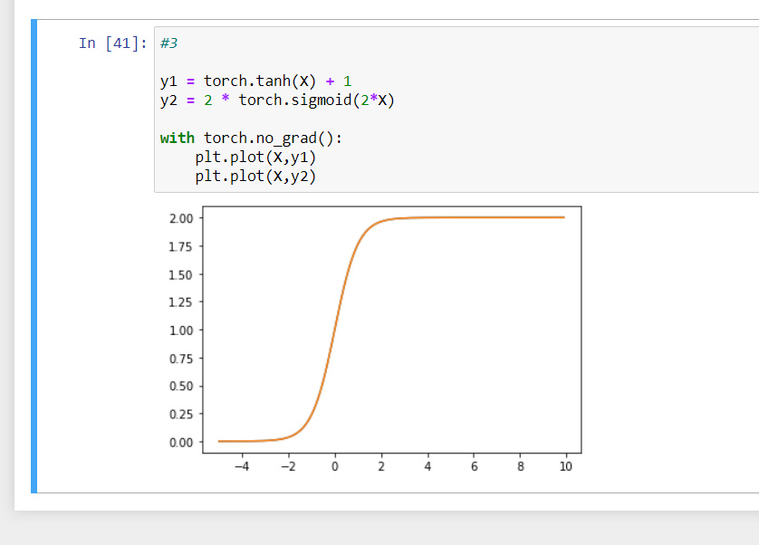
One linear functions add,minus other linear function still is linear function. - [1−exp(−2x)]/[1+exp(−2x)]+1 = 2/[1+exp(−2x)] = 2 * 1/[1+exp(−2x)] = 2 sigmoid(2x).
- d/2 dimensions will cause linearly dependent?
- overfit?
The section for plotting the gradient relu function.
y.backward(torch.ones_like(x), retain_graph=True)
d2l.plot(x.detach(), x.grad, ‘x’, ‘grad of relu’, figsize=(5, 2.5))
Should there be a
y.backward(torch.ones_like(x), retain_graph=True)
d2l.plot(x.detach(), x.grad, ‘x’, ‘grad of relu’, figsize=(5, 2.5))
x.grad.data.zero_()
Else if we run the notebook twice the gradient will keep on adding
Sure @sushmit86 that’s a genuine concern and would be a good idea but we don’t want to add complexity to the book content.
If you feel the need to run the cells twice you can add the extra line to zero out the grads 
Thanks so much for the reply
Question 2:
I think it should be this:
- H = Relu(XW^(1) + b^(2))
- y = HW^(2) + b^(2)
More detail in page 131.
I think it is more easy to think like this:
Relu(x) constructs a continuous piecewise linear function for every x\in R. So, it do not depend on whatever x is providing that x is continuous in R. So, Relu(Relu(x)*W+b) for example is also constructs a continuous piecewise linear function.
Question 4:
I think the most different between an MLP apply nonlinearity and MLP not apply nonlinearity is the time and complexity. In fact, MLPs applying nonlinearity such as Sigmoid and tanh are very expensive to calculate and find the derivative for gradient descent. So, we need something faster and Relu is a good choice to address these problem (6.x sigmoid).
Ans for question 4
I think if we apply different non linearity for different mini batches , as the activation function changes the first thing is the range of the output will vary which we affect the final output
My answers
Exeercises
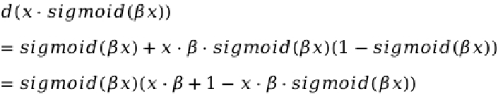
- Compute the derivative of the pReLU activation function.
- made a way to describe the function but the torch autograd is not able to work
alpha = 0.1
y = find_max(X) + alpha * find_min(X)
2. Show that an MLP using only ReLU (or pReLU) constructs a continuous piecewise linear
function.
- I guess we need to construct a multi layer perceptron here. dontknow.
- Show that tanh(x) + 1 = 2 sigmoid(2x).
- through plottinga graph we can show.
- Assume that we have a nonlinearity that applies to one minibatch at a time. What kinds of
problems do you expect this to cause?
- maybe this would create problems like each min batch would be squished(scaled) differently.
Hi, @goldpiggy
I have a question regarding eq (4.1.1), consequently the rest.
If X is a n *d matrix and W^(1) is a d *h matrix, then both H and XW^(1) is a n*h matrix. However, b^(1) is a 1*h row vector? The dimension of this equation is not consistent. Should it be b^(1) is a n*h matrix?
Similarly for b^(2)
Does deep learning framwork (like PyTorch, Tensorflow, …) use some tricks when calculating the derivative like sigmoid, tanh (exponential family) ? ![]()
D sigmoid(x) = sigmoid(x) * (1 - sigmoid(x)) can efficiently decrease computational work even if they use computational graph with backpropagation.
However, this also reduces the portability of the framework.
Here are my opinions for the exercises:
I don’t know the answer for ex.6 ![]()
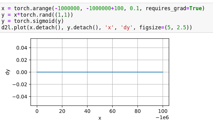
ex.1
The derivative for any x in a multi-layer perceptron nuralnetwork is always a fixed value, that is this kind of nn is always linear.
![]()
And if the weight of second layer has less dimensions than the first, the dimension of W model is reduced, which means a reduction of expressive capacity.
ex.2
![]()
ex.3
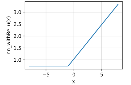
ex.4
x_1 = torch.arange(-8.0, 8.0, 0.1)
w_1 = torch.rand(1, 1)
b_1 = torch.rand(1, 1)
y_1 = x_1*w_1+b_1
x_2 = torch.relu(y_1)
w_2 = torch.rand(1, 1)
b_2 = torch.rand(1, 1)
y_2 = x_2*w_2+b_2
d2l.plot(x.detach(), y_2.detach(), 'x', 'nn_withReLu(x)')
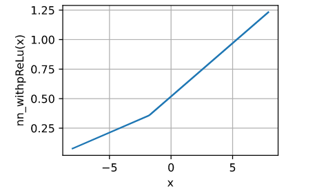
x_1 = torch.arange(-8.0, 8.0, 0.1)
w_1 = torch.rand(1, 1)
b_1 = torch.rand(1, 1)
y_1 = x_1*w_1+b_1
x_2 = torch.prelu(y_1,torch.tensor(0.5))
w_2 = torch.rand(1, 1)
b_2 = torch.rand(1, 1)
y_2 = x_2*w_2+b_2
d2l.plot(x.detach(), y_2.detach(), 'x', 'nn_withpReLu(x)')
ex.5
A. ![]()
B. As shown in A, tanh(x) is kinda like adding a affine layer just behind the activation stage with sigmoid , and considering the conclusion in ex1, this kind of affine layer can merge with the affine layer behind to make it identical to a nn using sigmoid, vice versa.
ex.6
??
ex.7
I have a really simple question. What does “q” denote in the section 5.1.1.3. From Linear to Nonlinear? The other variables are explained, but not this one. Thanks.
@Sintrias This confused me as well! See section 4.1.1.3.
“q” denotes the number of categories in the output. Thus,
- W(2) will be h x q weights → h weight vectors with weights for each of the q categories
- b(2) will be 1 x q weights → 1 bias for each of the q categories
- O will be n x q → n output vectors with values for each of the q categories
I am not sure about Eq. (5.1.8). If you run
y = (1-torch.exp(2*x))/(torch.exp(2*x)+1)
d2l.plot(x.detach(), y.detach(), 'x', 'tanh(x)', figsize=(5, 2.5))
you get the negative of
y = torch.tanh(x)
d2l.plot(x.detach(), y.detach(), 'x', 'tanh(x)', figsize=(5, 2.5))
Also, wikipedia says it should be the negative: Hyperbolic functions - Wikipedia.