Hello, is the correct answer to question 2 , part 3 …the plot of training and generalization loss against the amount of data ( losses versus data ) should be similar to the ones versus the modle complexity (losses versus the model complexity)
In section 4.4.4.5 Higher-Order Polynomial Function Fitting (Overfitting) the test error is quite similar to the training error. We hardly see any gap between test vs training error. Ideally, we should have seen a higher test error rate and a gap between training and test error. Let me know if my inferences are correct?
question1: w_i = y/(\sum x^i)
question 2: after 2 degrees, both reach nearly zero error
def train_2(train_features, test_features, train_labels, test_labels,
num_epochs=400):
loss = nn.MSELoss()
input_shape = train_features.shape[-1]
# Switch off the bias since we already catered for it in the polynomial
# features
net = nn.Sequential(nn.Linear(input_shape, 1, bias=False))
batch_size = min(10, train_labels.shape[0])
train_iter = d2l.load_array((train_features, train_labels.reshape(-1,1)),
batch_size)
test_iter = d2l.load_array((test_features, test_labels.reshape(-1,1)),
batch_size, is_train=False)
trainer = torch.optim.SGD(net.parameters(), lr=0.01)
for epoch in range(num_epochs):
    d2l.train_epoch_ch3(net, train_iter, loss, trainer)

return (evaluate_loss(net, train_iter, loss),
        evaluate_loss(net, test_iter, loss))
train_losses = []
test_losses = []
for i in range(1, len(poly_features[0]) + 1):
train_loss, test_loss = train_2(poly_features[:n_train, :i], poly_features[n_train:, :i], labels[:n_train], labels[n_train:])
train_losses.append(train_loss)
test_losses.append(test_loss)
bascially it is telling us the complexity will reduce the error and go to overfitting once beyond a point
1 Like
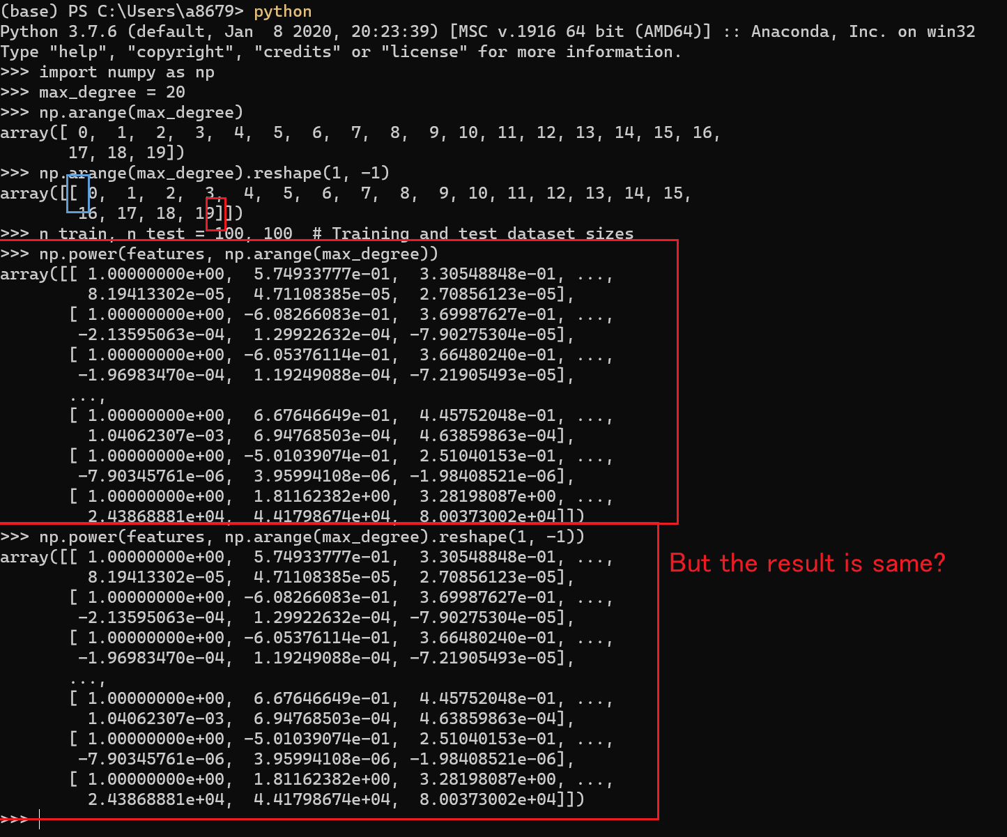
poly_features = np.power(features, np.arange(max_degree).reshape(1, -1))
why did we use reshape here
Hi! In Section 4.4.3, under “Model complexity”, it reads “In fact, whenever the data examples each have a distinct value of x, a polynomial function with degree equal to the number of data examples can fit the training set perfectly.”. Although this is true, it could be a little misleading to the unaware reader, who might, for example, think that a second-degree polynomial is needed to perfectly fit two data points, whereas a linear function would suffice. Therefore, it could be more general to say that “[…] a polynomial function with degree d >= n - 1 can fit the training set perfectly, where n is the number of data examples.”.
Great book! =)
Hello, when I try to solve the third question:
3. What happens if you drop the normalization (1/i!1/i!) of the polynomial features xixi? Can you fix this in some other way?
I found that I cannot get the answer when I increase the degree of the model to 6 or greater because of the explosion of gradient. I tried to fix it by decrease the learning ratio(1e-4) and increase the training epochs(1000) but got only little improvements (3.3 training error and 9.7 test error).
I wonder whether it is the right way to fix the problem or we have some other better solutions.
1 Like
Exercises and my attempt
- Can you solve the polynomial regression problem exactly? Hint: use linear algebra.
- dont know how to do it. exactly.
-
Consider model selection for polynomials:
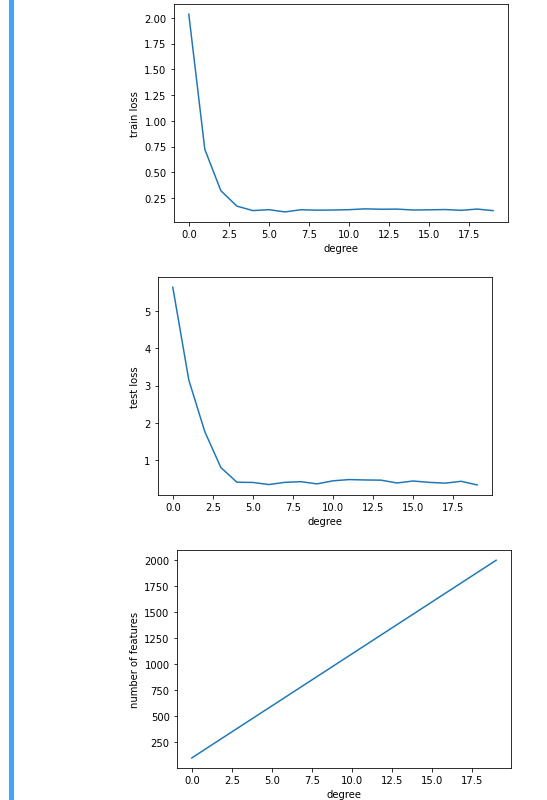
- Plot the training loss vs. model complexity (degree of the polynomial). What do you
observe? What degree of polynomial do you need to reduce the training loss to 0?
at about 5 degree it becomes zero.-
Plot the test loss in this case.
-
Generate the same plot as a function of the amount of data.
- plots for three:
- What happens if you drop the normalization (1/i!) of the polynomial features x
? Can you fix this in some other way?
-
the test loss and train loss become nan after 7th feature.
-
Maybe we can put our own normalisation feature mechanism, though I am not sure.
- Can you ever expect to see zero generalization error?
- only when the environment conditions are fully known.
this is a nice attempt
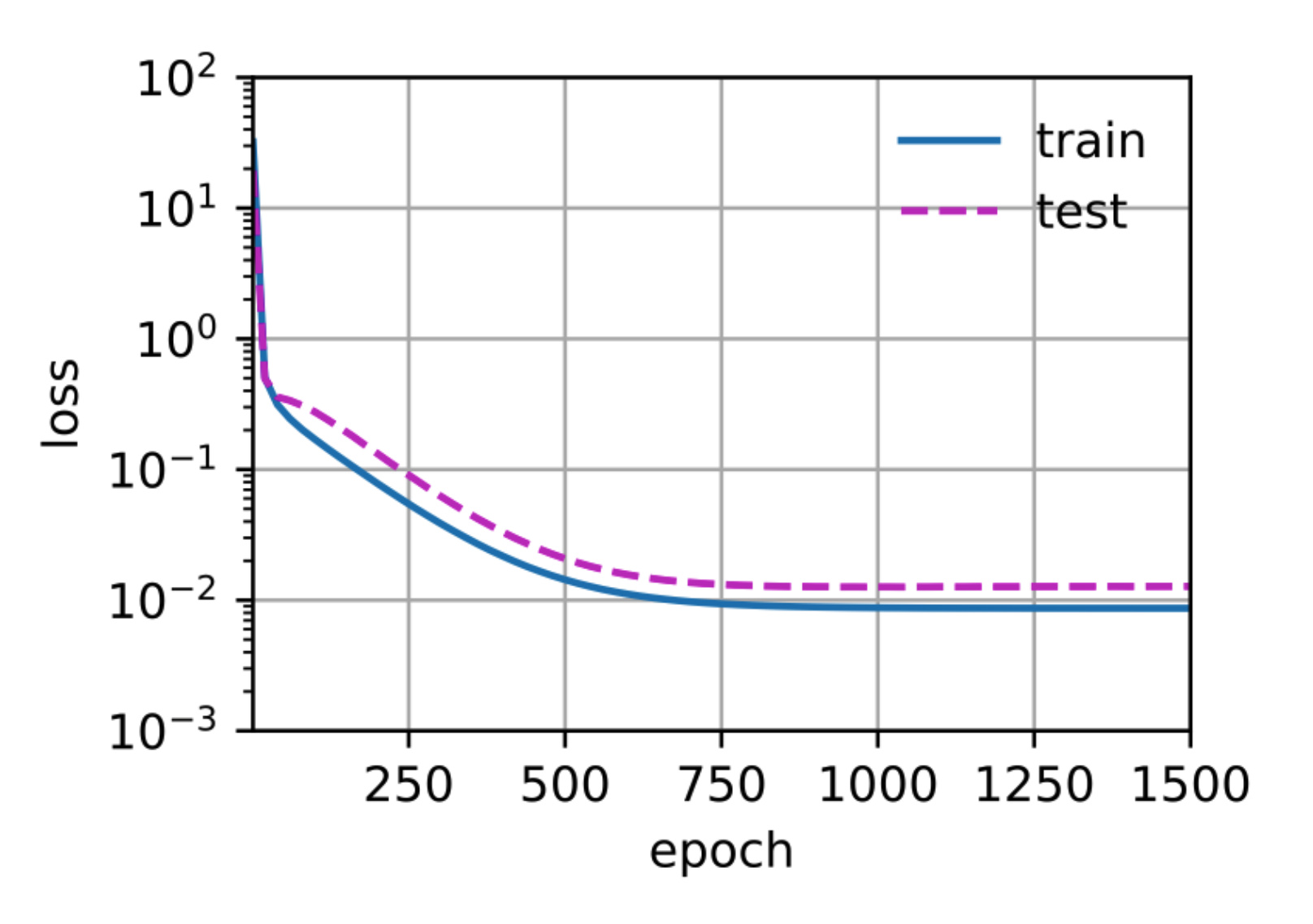
why this plot overfitting? I don’t understand, the training loss and testing loss decreases constantly to 0.01, and there’s no bounce-back of testing loss at the optimal point. To me, this plot shows a very successful training outcome.
I got following error when running the code, am I the only one? I am running using VS
PS C:\Users\T929189\PycharmProjects> & C:/Users/T929189/AppData/Local/Programs/Python/Python39/python.exe “c:/Users/T929189/PycharmProjects/Deep Learning/4.4_MPL_v1.1.py”
Traceback (most recent call last):
File “c:\Users\T929189\PycharmProjects\Deep Learning\4.4_MPL_v1.1.py”, line 56, in
train(poly_features[:n_train, :4], poly_features[n_train:, :4],
File “c:\Users\T929189\PycharmProjects\Deep Learning\4.4_MPL_v1.1.py”, line 48, in train
d2l.train_epoch_ch3(net, train_iter, loss, trainer)
File “C:\Users\T929189\AppData\Local\Programs\Python\Python39\lib\site-packages\d2l\torch.py”, line 271, in train_epoch_ch3
l.backward()
File “C:\Users\T929189\AppData\Roaming\Python\Python39\site-packages\torch\tensor.py”, line 245, in backward
torch.autograd.backward(self, gradient, retain_graph, create_graph, inputs=inputs)
File “C:\Users\T929189\AppData\Roaming\Python\Python39\site-packages\torch\autograd_init_.py”, line 141, in backward
grad_tensors_ = make_grads(tensors, grad_tensors)
File “C:\Users\T929189\AppData\Roaming\Python\Python39\site-packages\torch\autograd_init_.py”, line 50, in _make_grads
raise RuntimeError(“grad can be implicitly created only for scalar outputs”)
RuntimeError: grad can be implicitly created only for scalar outputs
It works by changing to loss=nn.MSELoss()
Add d2l.plt.show() to the end of train function, you will be able to see the generated chart.
May I know why the following line is needed?
np.random.shuffle(features)
It seems that
features = np.random.normal(size=(n_train + n_test, 1))
is already a random sequence, so shuffle is unnecessary.
Thanks!
- What happens if you drop the normalization (1/i!) of the polynomial features xi? Can you fix this in some other way?
As for the third question, the parameters of net will be NAN(too large). It’s because some of the features may be larger than 1, giving rise to tremendous poly feature value. When updating parameters with sgd, the huge poly feature values will make the weights grow to unacceptably large.(You can calculate the derivatives of the loss function to check this)
My way to fix this is just to make all the features smaller than 1. I just divide all the features by 1000 and it works!
Here are my opinions about exs:
These exs are indefinitive, so I’m not sure about my answers…
ex.1
I think if all the dimension of data is independent, we can work out every w exactly.
ex.2
- If I do a survey of “how long do you sleep at night”, I collect the answer in different season, but didn’t count the season as a dimension, then I a loss an important dimension.
- I ask the question in ex.1 on somebody once more, then the model I trained may biased on the repeateable example.
- The handwriting images taken from one single person will train out a model not capable of predict everyone’s handwriting.
- The ruler I evaluate somebody’s height shrink in the low temperature, then the data may depend on temperature where I didn’t mention in any dimension.
- I want to research the relation between the ear length and weight of wild rabbit, I try to catch some rabbit and weight them, but some stronger(weight more) one is missed, that means my model will biased on little rabbit.
ex.3
1.I train myself to remember 100 questions and it’s answer I met in the past, without understanding why, then the nuerons in my brain may be trained to detect each questions, say, I got 100 buerons, where each one reperesents if a question appears.
If I see a old question, I will know witch one it is, then I may choose the answer of the relative question without an error.
So if I have a model that is complicate to differentiate each example in my training set, I will get a 0 training error.
ex.4
Because the cumputation of training error and validation error on a same number of examples will take K times as before(For each example, it is used K times rather than only once).
ex.5
Because each example play two roles of both trainer and validator, like self-justifying, and that may cause overfitting more easily.
ex.6
I think the VC dimension only tell qualitative ability but not quantitative ability, for example, it can tell the difference bwteen apple and pear, but can’t tell how dilicious the apple or pear is.
ex.7
I may decrease the data set to a easy one(merge some categories to one, use less dimensions), and use my algorithm to perform a better result, thus prove to my manager that the structure of my algorithm is appropriate for this kind of data, in another word, my model is good enough. Then he may know that the problem is the size of data.
1 Like
Hi - thanks for a very good book! Not sure if there’s a discussion area for references, but I was struck by the Popper reference near the beginning - Popper-2005. The reference is the quite famous book by Karl Popper - “The logic of scientific discovery.” There may have been some recent edition published in 2005, but the book was first published in 1959. The 2005 date took me by surprise because Popper died in 1994.
Is there any mathematical proof for the fact that training error is a biased estimate of the generalization error? I think in the limit of infinite training data (maybe even when the finite traning set is representative of the population?), then it would be no longer biased.
- You can solve the problem of polynomial regression exactly when our design matrix is invertible - this requires we have at least as many distinct data points as parameters and that those points not make the columns linearly dependent.
- Time series price data for stocks. Disease transmission during an epidemic. Predicting the weather. Predicting masked pixels in an image. Predicting words in a sentence.
- You can expect zero training error given a sufficiently simple dataset or a model with extremely high capacity trained long enough to “memorize” the data. You’d only expect to see zero generalization error in strictly deterministic systems.
- Because you need to train (and validate) K models!
- Because the model’s trainer is likely using the results to maker hyperparameter and modeling choices, and there isn’t any holdout data to use thereafter. The model also isn’t being trained on all of the data, which might lead to slightly weaker models on average.
- The VC dimension captures a certain component of complexity, but doesn’t capture the range of values a function is allowed to take on very well.
- Demonstrate the relationship between data and performance up to the amount I currently have - if the trend is clearly positive, it indicates that we’d benefit from more data!