https://d2l.ai/chapter_linear-regression/linear-regression-scratch.html
Hello, I have a doubt about the visualization part.
My understanding:
Here, the data was generated according to a normal distribution of mean 0 and stddev 1.
Number of samples generated = (1000 x 2) = 2000 samples.
By a sample, I mean one scalar value.
These 2000 samples are then reshaped according to the size given.
The given size is (1000 x 2), therefore, I will end up with a matrix with 2 columns and 1000 rows.
When I visualize each column (1000 x 1) with respect to y, I get the following scatter plot:
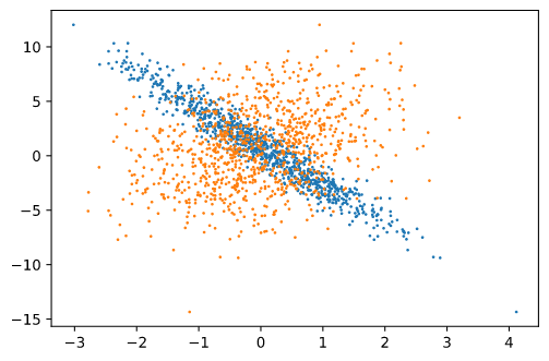
Each color represents a column. The y axis is labels and X-axis corresponds to column 1 and column 2, of features.
The visualization of one column matches with the text reference.
Expectation:
Since both columns correspond to independent variables, I do not understand why one of them is concentrated and the other is more spread out. Shouldn’t both follow the same pattern?
Relevant code
true_w = np.array([1.0, -3.4]).reshape(-1, 1)
true_b = np.array([0.8])

def generate_data(w, b, num_rows):
    """Generate y = Xw + b + noise."""
    X = np.random.normal(0, 1, (num_rows,len(w)))
    y = np.dot(X, w) + b
    y += np.random.normal(0, 0.01, y.shape)
    return X, y.reshape((-1, 1))

X,y = generate_data(true_w, true_b, 1000)

import matplotlib.pyplot as pl
plt.scatter(X[:, 1], y, 1)
plt.scatter(X[:, 0], y, 1)Answering my own question 
That is because of the values of w.
We know, y = w1x1 + w2x2 + b
How much each variable influences the output is dependent on the weight associated with it.
In my example: w1 = 1.0. w2 = -3.4, which means influence of w2 is higher than w1. (more than three times, even though in the opposite direction). Therefore, when I plot x2 and y, since x2 has a higher inflluence through w2, the straight line characteristic of y is more pronounced.
(I tried various values of w1 and w2 and checked how the graph is coming up)
Infact, the slope of the line is proportional to the ratio of the coefficient of the variable in x-axis to that of the other variable.
i.e, if I am plotting wrt x2, then slope of y (as obtained in the graph) is proportional to w2/w1.
If I am plotting wrt x1, then slope of y (as obtained in the graph) is proportional to w1/w2.
That is why, for the first variable, the “straight-line” effect is less pronounced.
The surface graph (x1 and x2 vs y) comes out to be a plane, as expected!
Great visualization!
 Good point. In short, the coefficient will scale the volatility.
Concerning question of Planck density temperature distribution, I may have an answer .
The distribution of temperature as a function of frequency is a bell-shaped curve.
A nonlinear transformation, like the Cox-Box transformation, aims to bring this distribution back to a normal distribution.
Maximize the likelihood probability P (T | L) of this normal law, where T is the temperature and L the wavelength, therefore, the energy of the radiation amounts, leads to calculate the solution of an optimization problem using least squared method.
It is therefore possible to use Planck’s distribution law to predict the temperature as a function of its spectral energy density.
1 Like
Any answer for automatic second derivative?
My guess is that computing 2nd derivative computes a large array of computations(by infinitesimal delta) around the point where we want to get the 2nd derivative to ensure the function(1st derivative) is continuous and differentiable. And then another loop to compute the 1st derivative of 1st derivative. So effectively O(1st derivative)*O(1st derivative is differentiable).
1 Like
Hi there. First off, fantastic work on all the D2L assets!
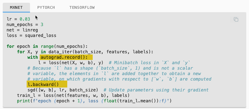
My question is related to the MXNet (really all frameworks) in the code example of linear regression from scratch. Specifically the use of the MXNet.autograd package.
The ASK: Are there examples of the linear-regression-scratch code that do not use MXNet and just use straight python? For example, the training loop in section 3.2.7 uses autograd.record() and backward(). Also “w” and “b” are initialized with attach_grad(). See highlight in pics below.
I realize implementing without a framework might be super inefficient, however, for better learning of Linear Regression and Gradient Descent algorithms, it would be interesting to see an implementation in straight python without an ML Framework.
Many thanks in advance for guidance on implementing the example code without MXNet or other ML Frameworks.
Well, as the name suggest you take gradient ∇L(ŷ(X,w,b),y) where L=loss(ŷ,y) and ŷ=net(X,w,b)
∇L(ŷ(X,w,b),y)= [∂L/∂ŷ,∂L/∂y]= [(∂L/∂X,∂L/∂w,∂L/∂b),∂L/∂y]. However from this gradient we are only interested in derivatives of parameters w and b. ∂L/∂w=∂L/∂ŷ•∂ŷ/∂w and ∂L/∂b=∂L/∂ŷ•∂ŷ/∂b. Calculation is easy: ∂L/∂ŷ=ŷ-y, ∂ŷ/∂w=X and ∂ŷ/∂b=1. So ∂L/∂b=∂L/∂ŷ, ∂L/∂w=X.T•∂L/∂ŷ. Then we need to rewrite the update function as well because we will no longer have the grad property available.
dldyh = net(X, w, b) - y.reshape(-1,1) # der. of square loss
b_grad= dldyh.sum(axis=0)               # dldb
w_grad= X.T.dot(dldyh)                     # dldw

sgd_d([w, b],[w_grad, b_grad], lr, batch_size)

def sgd_d(params, params_grad, lr, batch_size):
    for i, param in enumerate(params):
        param[:] = param - lr * params_grad[i] / batch_size