Because typically a vector is considered as a column vector. So $\mathbf{a}^T=[a_0, a_1, a_2, \cdots, a_n]$ ($\mathbf{a}^T$ becomes a row vector.). Now if you expand each element, you get the original matrix.
Ex1-3.
-
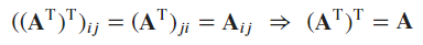
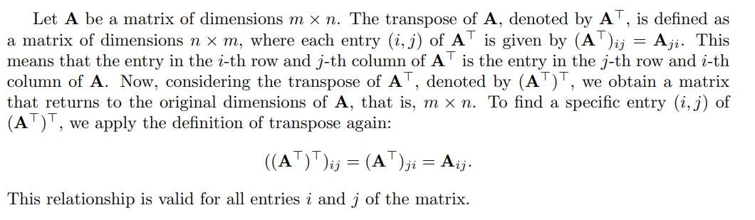
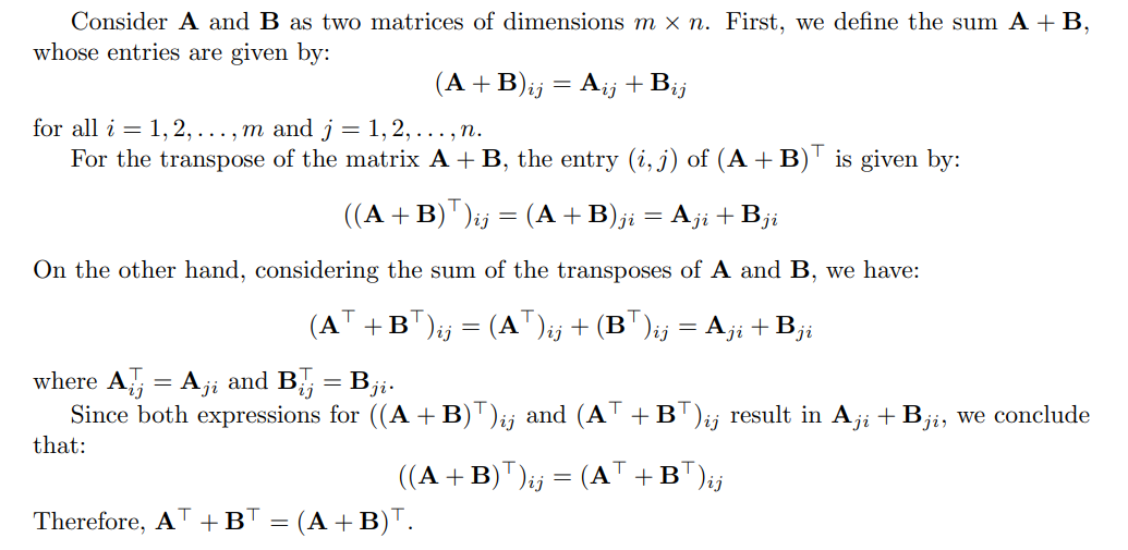
The transpose of transpose
-
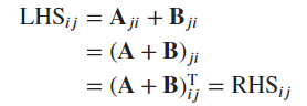
Commutativity of transpose and addition
-
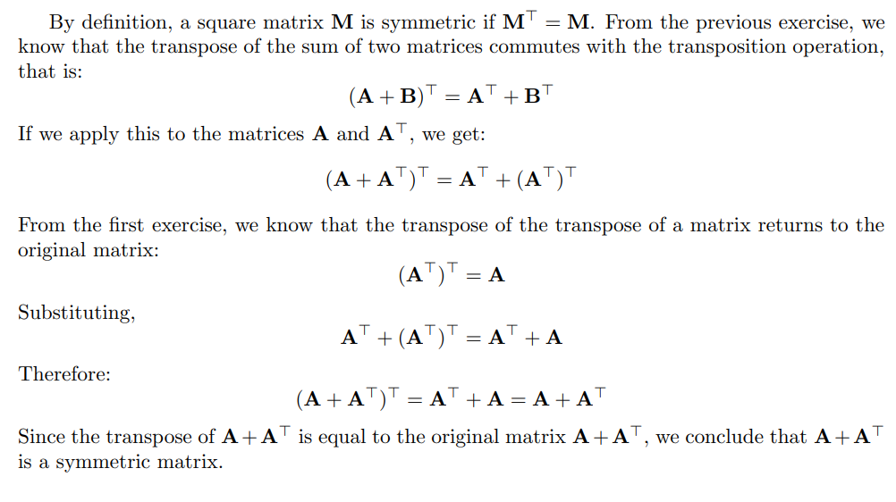
Symmetrization of a matrix
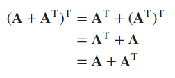
- The first equality is based on Ex2 (commutativity), and the second equality is based on Ex1 (transpose of transpose);
- The last equality holds due to the commutativity of the addition operation
Ex4-5.
- The
len()method, similar to that in NumPy arrays, returns the first dimension of a given tensor. - The basis is the magic function
__len__implemented in the corresponding classes (e.g., arrays or tensors).
import torch
X = torch.arange(24).reshape(2, 3, 4)
len(X)
Output:
2
Ex6 & 8
A = torch.arange(6, dtype=torch.float32).reshape(2, 3)
A / A.sum(axis=1)
Output:
---------------------------------------------------------------------------
RuntimeError                              Traceback (most recent call last)
Cell In[3], line 2
      1 A = torch.arange(6, dtype=torch.float32).reshape(2, 3)
----> 2 A / A.sum(axis=1)

RuntimeError: The size of tensor a (3) must match the size of tensor b (2) at non-singleton dimension 1
- The size of
Ais(2,3), andA.sum(axis=1)yields a reduced summation tensor in shape(2, ).- With two tensors of different numbers of axes (different dimensionalities), neither the direct element-wise operation
/nor its broadcast version can be performed.
- With two tensors of different numbers of axes (different dimensionalities), neither the direct element-wise operation
A.shape, A.sum(axis=1).shape
Output:
(torch.Size([2, 3]), torch.Size([2]))
- The operation that this problem really “wants” to perform is probably a column-wise normalization, where each element
 is divided by the summation of all elements in the row where lies, so that each row of the resulting tensor sums up to 1. But since the particular dimension to sum has been reduced, the broadcasting scheme will fail.
- A solution: use
keepdims=Trueto preserve the axis. After the summation, the size of this axis will be 1, but not zero.
- A solution: use
A / A.sum(axis=1, keepdims=True)
tensor([[0.0000, 0.3333, 0.6667],
        [0.2500, 0.3333, 0.4167]])
- A closer look at the reduced summation operation
B = torch.arange(24).reshape(2, 3, 4)
B.shape, B.sum(axis=0).shape, B.sum(axis=1).shape, B.sum(axis=2).shape
Output:
(torch.Size([2, 3, 4]),
 torch.Size([3, 4]),
 torch.Size([2, 4]),
 torch.Size([2, 3]))
Ex7.
- In downtown Manhattan, streets are rectilinearly distributed, and one has to travel from point
 to
to  along a trajectory composed of only horizontal and vertical lines.
- In such a case, the shortest distance to travel is
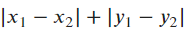 .
.
- In such a case, the shortest distance to travel is
- For a given space with dimension
 , the Manhattan distance between two points
  and
and  is defined as
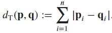
- This is applicable in signal processing, Machine Learning models, etc.
Ex9.
-
By default, the
torch.linalg.norm()function computes the Frobenius norm (for more-than-one ordered tensors) or the L2-norm (for one-ordered tensors, or vectors), as per the documentation.
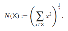
-
Below shows an example of a 4-ordered tensor
torch.manual_seed(706)
X = torch.randn(2, 3, 4, 5)
torch.linalg.norm(X), ((X ** 2).sum()) ** 0.5
Output:
(tensor(11.9074), tensor(11.9074))
Ex12.
A = torch.ones(100, 200, dtype=torch.int32)
B = torch.ones_like(A) * 2
C = torch.ones_like(A) * 3
stacked = torch.stack([A, B, C])
stacked.shape
Output:
torch.Size([3, 100, 200])
- By default, the
torch.stack()function constructs a new dimension at axis 0, along which the same-sized tensors are stacked, as per the documentation.- To slice out
B, one indexes1in the first axis.
- To slice out
(stacked[1] == B).sum() == B.numel()
Output:
tensor(True)
Exercise 10: let’s me clarify A,B and C they are same tensor dimension
# Pytorch
import time

# Define matrix dimensions
dim_A = (216, 216)
dim_B = (216, 216)
dim_C = (216, 216)

# Generate random matrices A, B, and C
A = torch.randn(*dim_A)
B = torch.randn(*dim_B)
C = torch.randn(*dim_C)

# Compute (AB)C and measure time and memory
start_time = time.time()
AB = np.dot(A, B)
ABC = np.dot(AB, C)
execution_time_ABC = time.time() - start_time
memory_usage_ABC = ABC.nbytes / (1024 * 1024)  # Convert bytes to MB

# Compute AC^T and measure time and memory
start_time = time.time()
AC_T = np.dot(A, C.T)
execution_time_ACT = time.time() - start_time
memory_usage_ACT = AC_T.nbytes / (1024 * 1024)  # Convert bytes to MB

# Print results
print("(AB)C:")
print("Execution time:", execution_time_ABC, "seconds")
print("Memory usage:", memory_usage_ABC, "MB")
print("\nAC^T:")
print("Execution time:", execution_time_ACT, "seconds")
print("Memory usage:", memory_usage_ACT, "MB")

Ouput:

(AB)C:
Execution time: 0.0015840530395507812 seconds
Memory usage: 0.177978515625 MB

AC^T:
Execution time: 0.0008935928344726562 seconds
Memory usage: 0.177978515625 MB
Time and space complexity
Note: space complexity = memory footprint
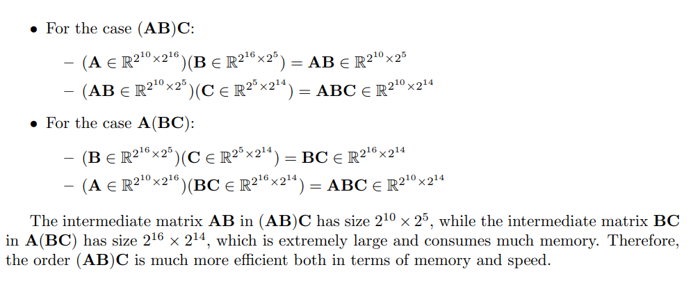
- $(AB)C$: They are require 2 times for matrix multiplication as $A$ multiplication $B$ and then $AB$ multiplication $C$ for matrix multiplication. If we are going deeper into the pseudo-code of matrix multiplication:
def multiply_2_matrix(matrix_a, matrix_b):
    rows_a = len(matrix_a)
    cols_a = len(matrix_a[0])
    rows_b = len(matrix_b)
    cols_b = len(matrix_b[0])

    if cols_a != rows_b:
        raise ValueError("Number of columns in matrix_a must match the number of rows in matrix_b")

    result = [[0] * cols_b for _ in range(rows_a)]

    # traveling through all rows of A
    for i in range(rows_a):
        # traveling through all columns of B
        for j in range(cols_b):
            # traveling through all columns of A
            for k in range(cols_a):
                # at any ij position = sum of i*k
                result[i][j] += matrix_a[i][k] * matrix_b[k][j]

    return result
So in matrix multiplication:
$;;;;$ Time complexity = 2 times of operation($A$ x $B$ and then $AB$ x $C$) is $O(i^2j)$ per 1 multiplication → In summary $O(i^2j)$
$;;;;$ Space complexity = $O(ij)$ (They not store new memory in next times operation just update result)
- $AC^T$: They are require 1 times for matrix multiplication as $A$ multi $C^T$ for matrix multiplication. If we are going deeper into the pseudo-code of transpose matrix:
def transpose_matrix(matrix):
    # New list of transpose matrix
    transposed = []
    # traveling through all columns
    for i in range(len(matrix[0])):
        transposed_row = []
        # update column as row
        for row in matrix:
            transposed_row.append(row[i])
        transposed.append(transposed_row)
    return transposed
So in matrix multiplication:
$;;;;$ Time complexity = 1 times of operation($A$ x $C^T$) is $O(i^2j) per 1 multiplication. And 1 times of transpose matrix of C in $O(ij)$. Even though time complexity of $AC^T$ = $(AB)C$ is $O(i^2j)$ but $O(ij)$ of transpose will less than $O(i^2j)$ of multiplication. → In summary $O(i^2j)$
$;;;;$ Space complexity = $O(ij)$ (Even $C^T$ will create new memory but just a tempory memory when multiplication with $A$ will update an store in result memory).
So that why $(AB)C$ need to spend more time $AC^T$ while memory footprint are equal.
My solutions. As a note – it would be nice if this forum had MathJax support! I’m also unable to include more than 2 links or 1 embedded media item as a new user.
Does anyone have a solid answer for #11?
- 2
len(x)always returns the length of the first (outermost) dimension.- There’s an error – but if you add
keepdim=True, this operation normalizes the columns (such that they add up to one). - Manhattan distance (avenues + streets), and sometimes (on Broadway or in the village)!
- (3, 4), (2, 4), and (2, 3) along axes 0, 1, and 2 respectively.
- It outputs the l2 norm for vectors, and the frobenius norm for matrices. For arbitrary tensors, it returns the square root of the sum of the squares of the tensor’s elements.
- For an m x k @ k x n matmul, you perform m * n * (m+n+1) FLOPs. k disappears! So (AB)C is faster than A(BC), since 16 > 5 (and you want to make the larger number “disappear”).
- I’m not sure about this one. There may be a greater overhead because of different memory access patterns, or some overhead associated with the tranpose itself. If that is the case, initializing C = B^\top would save the cost of memory duplication. I’m not sure what effect this would have on data access patterns.
3 x 100 x 200.
Exercise 1
import torch

A = torch.arange(6, dtype=torch.float64).reshape(2, 3)
(A.T).T == A
tensor([[True, True, True],
        [True, True, True]])
Exercise 2
B = A.clone()
A.T + B.T == (A + B).T
tensor([[True, True],
        [True, True],
        [True, True]])
Exercise 3
M = torch.arange(9, dtype=torch.float64).reshape(3, 3)
M + M.T == (M + M.T).T
tensor([[True, True, True],
        [True, True, True],
        [True, True, True]])
Exercise 4
The tensor X has the shape (2, 3, 4), meaning it has 2 elements in the first dimension, each being a tensor of shape (3, 4). Therefore, the output of len(X) is 2, as this function returns the size of the first dimension of a tensor.
X = torch.arange(24).reshape(2, 3, 4)
len(X)
2
Exercise 5
Yes, len(X) will always correspond to the length of the first axis (axis 0).
Exercise 6
try:
    A / A.sum(axis=1)
except Exception as error:
    print(A.shape, A.sum(axis=1).shape, error, sep="\n")
torch.Size([2, 3])
torch.Size([2])
The size of tensor a (3) must match the size of tensor b (2) at non-singleton dimension 1
Notice that A and A.sum(axis=1) have different dimensions, so the operation does not occur. The error, therefore, informs that the division requires the sum vector to be resized to match the dimensions of the original matrix. Like this:
A / A.sum(axis=1, keepdim=True)
tensor([[0.0000, 0.3333, 0.6667],
        [0.2500, 0.3333, 0.4167]], dtype=torch.float64)
Exercise 7
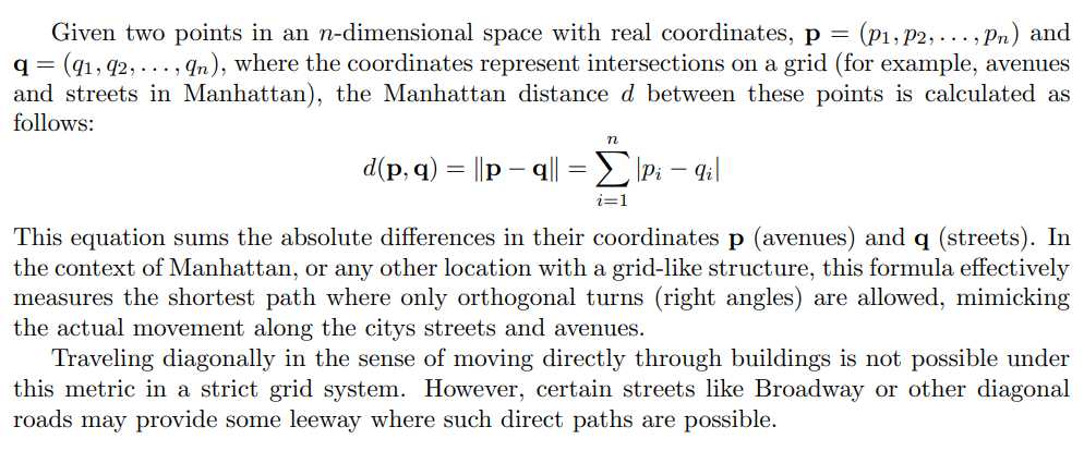
Source: Taxicab geometry and map of Manhattan Center.
Exercise 8
X = torch.arange(24).reshape(2, 3, 4)
X,X.sum(axis=0), X.sum(axis=1), X.sum(axis=2)
(tensor([[[ 0,  1,  2,  3],
          [ 4,  5,  6,  7],
          [ 8,  9, 10, 11]],

         [[12, 13, 14, 15],
          [16, 17, 18, 19],
          [20, 21, 22, 23]]]),
 tensor([[12, 14, 16, 18],
         [20, 22, 24, 26],
         [28, 30, 32, 34]]),
 tensor([[12, 15, 18, 21],
         [48, 51, 54, 57]]),
 tensor([[ 6, 22, 38],
         [54, 70, 86]]))
Exercise 9
X = torch.arange(24, dtype=torch.float64).reshape(2, 3, 4)
torch.linalg.norm(X)
tensor(65.7571, dtype=torch.float64)
torch.linalg.norm() computes the Frobenius norm for matrices (2D tensors) and the L2 norm for tensors with more than two dimensions. Thus, the previous result represents the magnitude of the vector in a high-dimensional space formed by flattening the tensor X. Applying this function “forcefully”:
def l2(tensor):
    return torch.sqrt(torch.sum(tensor ** 2))
l2(X)
tensor(65.7571, dtype=torch.float64)
Exercise 10
import psutil
import time

def memory(X, Y):
    start = time.time()
    torch.mm(X, Y)
    memory = psutil.virtual_memory()
    print(f"Total system memory: {memory.total / (1024 ** 3):.2f} GB")
    print(f"Memory used: {memory.used / (1024 ** 3):.2f} GB")
    print(f"Available memory: {memory.available / (1024 ** 3):.2f} GB")
    print(f"CPU usage: {psutil.cpu_percent():.2f}%")
    elapsed = time.time() - start
    print(f"Elapsed time: {elapsed:.2f} seconds\n")

torch.manual_seed(42)
A = torch.randn(2 ** 10, 2 ** 16, dtype=torch.float64)
B = torch.randn(2 ** 16, 2 ** 5, dtype=torch.float64)
C = torch.randn(2 ** 5, 2 ** 14, dtype=torch.float64)

memory(torch.mm(A, B), C)
memory(A, torch.mm(B, C))
Total system memory: 19.23 GB
Memory used: 2.82 GB
Available memory: 15.72 GB
CPU usage: 21.10%
Elapsed time: 0.05 seconds

Total system memory: 19.23 GB
Memory used: 10.82 GB
Available memory: 7.75 GB
CPU usage: 70.70%
Elapsed time: 27.60 seconds
Exercise 11
I believe there is a typographical error in this question because the operation torch(A, B.T) is not possible due to dimension incompatibility. In this case, I did C = C.T (which I think is what the authors actually intended).
torch.manual_seed(42)
C = torch.randn(2 ** 5, 2 ** 16, dtype=torch.float64)

memory(A, B)
memory(A, C.T)

C = C.T
memory(A, C)
Total system memory: 19.23 GB
Memory used: 3.26 GB
Available memory: 15.22 GB
CPU usage: 12.00%
Elapsed time: 0.07 seconds

Total system memory: 19.23 GB
Memory used: 3.28 GB
Available memory: 15.22 GB
CPU usage: 15.00%
Elapsed time: 0.06 seconds

Total system memory: 19.23 GB
Memory used: 3.27 GB
Available memory: 15.22 GB
CPU usage: 9.50%
Elapsed time: 0.07 seconds
-
Theoretically, the operations
torch.mm(A, B)andtorch.mm(A, C.T)should have similar performance in terms of computational complexity, but differ in memory access due to the data orientation ofC.T. It was expected that transposition would negatively affect efficiency due to non-sequential memory access. However, the time difference betweentorch.mm(A, B)andtorch.mm(A, C.T)is minimal. Perhaps the internal optimization of PyTorch for transpose operations is quite effective, minimizing the theoretically negative impact of memory transposition. -
Pre-transposing
Cand performing the multiplication withAshows a runtime comparable totorch.mm(A, B), with slightly reduced CPU usage. The reduction in CPU usage may be due to the elimination of the need for dynamic transposition during multiplication, indicating that pre-processingCmight be beneficial from the perspective of reducing CPU load, despite not significantly impacting runtime.
Exercise 12
torch.manual_seed(42)
A = torch.randn(100, 200, dtype=torch.float64)
B = torch.randn(100, 200, dtype=torch.float64)
C = torch.randn(100, 200, dtype=torch.float64)
torch.stack([A,B,C]).shape, torch.stack([A,B,C])[1] == B
(torch.Size([3, 100, 200]),
 tensor([[True, True, True,  ..., True, True, True],
         [True, True, True,  ..., True, True, True],
         [True, True, True,  ..., True, True, True],
         ...,
         [True, True, True,  ..., True, True, True],
         [True, True, True,  ..., True, True, True],
         [True, True, True,  ..., True, True, True]]))
2 Likes
I used:
# Problem 11
A = torch.rand(2**10, 2**16)
B = torch.rand(2**16, 2**5)
C = torch.rand(2**5, 2**16)
%timeit A @ B
%timeit A @ C.T
and got the following results:
27 ms ± 1.4 ms per loop (mean ± std. dev. of 7 runs, 10 loops each)
and
27.6 ms ± 337 µs per loop (mean ± std. dev. of 7 runs, 10 loops each)
respectively.
Why does everyone else seem to have the second one equal to or faster than the first one ?
1 Like
Seems like torch.linalg.norm(x) and torch.norm(x) give the same output irrespective of the shape & size of x.
If that is the case, why not just deprecate one of the them?
import psutil
import time

def memory_usage():
    memory = psutil.virtual_memory()
    print(f"Total system memory: {memory.total / (1024 ** 3):.2f} GB")
    print(f"Used memory: {memory.used / (1024 ** 3):.2f} GB")
    print(f"Available memory: {memory.available / (1024 ** 3):.2f} GB")

a = 2**10
b = 2**16
c = 2**5
d = 2**14

A = torch.randn(a*b).reshape(a,b)
B = torch.randn(b*c).reshape(b,c)
C = torch.randn(c*a).reshape(c,a)

print(f" {A.size()} X {B.size()} ")
T1 = A@B
print(f" {T1.size()} X {C.size()} ")
T2 = T1@C
memory_usage()
elapsed_time = time.time() - start_time
print(f"Elapsed time: {elapsed_time:.2f} seconds\n")

print(f" {B.size()} X {C.size()} ")
start_time = time.time()
T1 = B@C
print(f" {A.size()} X {T1.size()} ")
T2 = A@T1
memory_usage()
elapsed_time = time.time() - start_time
print(f"Elapsed time: {elapsed_time:.2f} seconds\n")
I also got A(BC) faster than (AB)C
torch.Size([1024, 65536]) X torch.Size([65536, 32])
 torch.Size([1024, 32]) X torch.Size([32, 1024])
Total system memory: 15.68 GB
Used memory: 9.96 GB
Available memory: 5.72 GB
Elapsed time: 59.86 seconds

 torch.Size([65536, 32]) X torch.Size([32, 1024])
 torch.Size([1024, 65536]) X torch.Size([65536, 1024])
Total system memory: 15.68 GB
Used memory: 10.22 GB
Available memory: 5.46 GB
Elapsed time: 0.98 seconds
Revisiting this chapter, I made a few mistakes:
6. If you add keepdim=True, this operation actually normalizes across the rows, not the columns.
- I’m not sure where I got this m*n*(m+n+1) idea. I worked this out using an example:
(2, 3) @ (3, 5) → (2*3-1) * 5 * 2
(m, k) @ (k, n) → (2k-1) * m * n FLOPs
A: (2^10, 2^16)
B: (2^16, 2^5)
C: (2^5, 2^14)
Using 2*m*k*n as an approximation:
(AB)C → 2^32 + 2^30 FLOPs = 5.37e9 FLOPs
A(BC) → 2^36 + 2^41 FLOPs = 2.27e12 FLOPs
(AB)C is ~422.4x fewer FLOPs
- My naive assumption was that although AB and AC^T have the same mathematical shape, taking C^T creates a strided array, which should lead to less efficient memory access. See:
x = torch.randn(200, 100)
print(x.stride(), x.T.stride())
Note: if you don’t know what stride is, see this excellent blog post on PyTorch internals.
Therefore, if you initialize C = B^T, C is just a view of the same underlying memory and the matmul will still be slower than AB. To fix this, call B.T.contiguous().
But when I benchmarked this, all three operations had practically the same speed:
(torch-env) f@mbp torch-env % python bench.py
Time per iteration (A @ B):           0.00221 s
Time per iteration (A @ C.t() view):  0.00226 s
Time per iteration (A @ cloned C^T):  0.00221 s
Here’s my benchmark code (ran on apple silicon macbook – you’ll have to modify it for other devices):
import torch
import time
import sys

if not torch.mps.is_available():
    print("Could not access mps device")
    sys.exit(1)

device = 'mps'

M = 2**10  #  1_024
K = 2**16  # 65_536
N = 2**5   #     32

# Test matrices A, B, C
A = torch.randn(M, K, device=device) # (2**10, 2**16)
B = torch.randn(K, N, device=device) # (2**16, 2**5)
C = torch.randn(N, K, device=device) # (2**5, 2**16)

def benchmark_matmul(matmul_fn, iters=1_000, warmup=100):
    # Warm up (not timed)
    for _ in range(warmup):
        _ = matmul_fn()
    torch.mps.synchronize()

    start = time.time()
    for _ in range(iters):
        out = matmul_fn()
    torch.mps.synchronize()
    end = time.time()

    return (end - start) / iters

# 1) Plain A @ B
time_ab = benchmark_matmul(lambda: A @ B)

# 2) A @ C.t(). C.t() is just a view, not copied.
time_ac_view = benchmark_matmul(lambda: A @ C.t())

# 3) A @ cloned transpose of C. Ensures contiguous memory.
C_t_contig = C.t().contiguous()
time_ac_cloned = benchmark_matmul(lambda: A @ C_t_contig)

print(f"Time per iteration (A @ B):           {time_ab:.5f} s")
print(f"Time per iteration (A @ C.t() view):  {time_ac_view:.5f} s")
print(f"Time per iteration (A @ cloned C^T):  {time_ac_cloned:.5f} s")
- You can perform this as follows:
A, B, C = torch.randn(3, 100, 200)
print(A.shape, B.shape, C.shape)
s = torch.stack([A, B, C])
print(s.shape)
print(f"B {'matches' if (s[1] == B).all().item() else 'does not match'}")
2.3.13 Exercises
Q1
matricA = torch.arange(6).reshape(3,2)
matricA
tensor([[0, 1],
        [2, 3],
        [4, 5]])
tmat = matricA.T
tmat
tensor([[0, 2, 4],
        [1, 3, 5]])
tmat.T, tmat.T == matricA
(tensor([[0, 1],
         [2, 3],
         [4, 5]]),
 tensor([[True, True],
         [True, True],
         [True, True]]))
2.3.13 Exercises
Q2
tsum = matricC.T + matricB.T
sumt = (matricC + matricB).T
tsum == sumt
tensor([[True, True, True],
        [True, True, True],
        [True, True, True],
        [True, True, True]])
Note: There should be atleast one dimension that should be same just like broadcasting for it to work, else it will give error!!
Q3
matricD = torch.tensor([[0,1,2], [1,4,5],[2,5,8]])
matricD
tensor([[0, 1, 2],
        [1, 4, 5],
        [2, 5, 8]])
matricD.T == matricD
tensor([[True, True, True],
        [True, True, True],
        [True, True, True]])