https://d2l.ai/chapter_appendix-mathematics-for-deep-learning/geometry-linear-algebraic-ops.html
The classifier used in the text seems rather unnatural. A more natural way is to flatten the images, normalize them, then take the dot product as discussed in the text as a measure of similarity. The predicted label is the label of the average image that is more similar to the test image, hence the argmax.
# normalize matrices using broadcasting
W = torch.stack([ave_0.flatten().t(), ave_1.flatten().t()], dim=1)
W = W / torch.norm(W, dim=0).reshape(1, -1)
X_test = X_test.reshape(-1, 784)
X_test = X_test / torch.norm(X_test, dim=1).reshape(-1, 1)

# predict and evaluate
y_pred = torch.argmax(X_test @ W, dim=1)
print((y_test == y_pred).type(torch.float).mean())
This obtains an accuracy of ~0.95. 
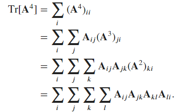
What’s the interpretation of A^4 in exercise 7?
I’ve typed up solutions to the exercises in this chapter here (see bottom of the notebook). I’m still seeking guidance on exercise 7.
Any help will be greatly appreciated!
Hey, maybe a little late here; but as far as I understand it, A^4 means a matrix with 4 dimensions.
Based on this section, I think A^4 means A * A * A * A, that is, matrix A multiplied 4 times by itself. It’s the power operator (A to the power of 4) for matrices, if I’m not mistaken.
In Section 18.1.3. Hyperplanes, it says - “The set of all points where this is true is a line at right angles to the vector w”. Which condition is “this” referring to here? Is it referring to all vectors (or rather, points here) whose projection is equal to 1/||w||?
# Accuracy\n torch.mean(predictions.type(y_test.dtype) == y_test, dtype=torch.float64)
Hi, I think the way to calculate the accuracy is not right here, since the predictions.type(y_test.dtype)==y_test will return a tensor which only contain the Boolean values. It can not be calculated by the torch.mean() function. So I think the right format should be:
torch.mean((predictions.type(y_test.dtype) == y_test).float(), dtype=torch.float64)
In this way the result is exactly the same.
Hi @Tate_Zenith,
Yes, the current implementation will raise a runtime error with the latest version of torch==1.10.2. This behaviour was fine if you try to run with torch==1.8.1.
I’ll send a fix to support the latest version. We’re working on making the master branch support the latest versions of all the frameworks.
That’s sounds great, thanks!
Section 18.1.6:
… C has rank two since, for instance, the first two columns are linearly independent, however any of the four collections of three columns are dependent.
Questions/doubts:
- Which four collections of three columns? There are 5C3=10 collections of 3 columns each that can be formed from the 5 columns. So, which 4 out of the 10 are being discussed here?
- Perhaps, it can be made clearer by giving the proof of linear dependence of one of the collections.
@ToddMorrill
For exercise7, this is what I think the solution is:
PS. this solution concern A^4 as a matrix multiplication and not element wise multiplication.
D = A^4 = A^2.A^2 = B^2
tr(D) = {sum, i} d_ii
dii = {sum, j} b_ij*b_ji
bij = {sum, k} a_ik*a_kj
dii = {sum, j}({sum, k}a_ik*a_kj)*({sum, l}a_jl*a_li)
dii = {sum, j}{sum, k}{sum, l}a_ik*a_kj*a_jl*a_li
tr(D) = {sum, i}{sum, j}{sum, k}{sum, l}a_ik*a_kj*a_jl*a_li
tr(A^4) = torch.einsum('ik,kj,jl,li', A, A, A, A)
I verified this answer with random matrices and it worked
size = 4
A = torch.randint(1, 100, (size, size))
tr_A_4 = torch.trace(torch.matmul(torch.matmul(A, A), torch.matmul(A, A)))
tr_A_4_einsum = torch.einsum('ik, kj, jl, li', A, A, A, A)
assert  tr_A_4 == tr_A_4_einsum
hope this can help you out:
torch.einsum(“ij,jk,kl,lm → im”, A,A,A,A).trace()
I don’t really understand the Tensors and Common Linear Algebra Operations subsection. The sum at 22.1.32 is a bit confusing.
Ex1.
- Using the function
angle(), we compute

def angle(x, y):
    """
    Computes the angle between two vectors.
    """
    return torch.acos(x.dot(y) / (torch.linalg.norm(x) * torch.linalg.norm(y)))
rad = angle(
    torch.tensor([1, 0, -1, 2], dtype=torch.float32),
    torch.tensor([3, 1, 0,  1], dtype=torch.float32)
)
rad, rad / 3.14 * 180
Output (in rad and degree, respectively):
(tensor(0.9078), tensor(52.0412))
Ex2.
- True. We can verify straightforwardly by definition.
M1 = torch.tensor([[1, 2], [0, 1]])
M2 = torch.tensor([[1, -2], [0, 1]])
M1 @ M2, M2 @ M1
Output:
(tensor([[1, 0],
         [0, 1]]),
 tensor([[1, 0],
         [0, 1]]))
Ex3.
- The determinant is the scaling factor of the transfomred area. We compute the determinant of the transform matrix:
torch.det(torch.tensor([[2, 3], [1, 2]], dtype=torch.float32))
Output:
tensor(1.)
- Since the determinant is 1, the area is left unchanged as 100.
Ex4.
- Linear independence is equivalent to a non-zero determinant.
- Below shows that only the first set of vectors is linearly independent.
is_linear_indep = lambda X: bool(torch.det(X))
X1 = torch.tensor([[1, 2, 3], [0, 1, 1], [-1, -1, 1]], dtype=torch.float32)
X2 = torch.tensor([[3, 1, 0], [1, 1, 0], [1, 1, 0]], dtype=torch.float32)
X3 = torch.tensor([[1, 0, 1], [1, 1, 0], [0, -1, 1]], dtype=torch.float32)
is_linear_indep(X1), is_linear_indep(X2), is_linear_indep(X3)
Output:
(True, False, False)
Ex5.
- It is true. By definition,

Ex6.
- We take the dot product,

Denoting , one has the condition for orthogonality which reads

Ex7.
-
We hierarchically “expand” the summation according to the definition of matrix multiplication:

- The corresponding Einstein summation notation should be
ij, jk, kl, li ->, where an empty string is used to represent a scalar.
- The corresponding Einstein summation notation should be
# Check our result
torch.manual_seed(706)
A = torch.randn(3, 3)
einsum = torch.einsum("ij, jk, kl, li ->" , A, A, A, A)
manual = torch.trace(A @ A @ A @ A)
einsum.item(), manual.item()
Output:
(141.1223907470703, 141.12237548828125)
The visualization at the start of 22.1.3. Hyperplanes in the image “Fig. 22.1.5 Recalling trigonometry, we see the formula ‖𝑣‖cos(𝜃) is the length of the projection of the vector 𝑣 onto the direction of 𝑤” is not accurately representing the 𝑦=1−2𝑥 equation. The line should intersect the y-axis at (0, 1), not at (0, 2) as shown.