@goldpiggy I don’t understand how underfitting is happening when we limit our polynomial degree to 3. I understand that the labels that we generated were made using poynomial of degree 4 and we are trying to train the 3 degree polynomial to get labels that are close to those generated by 4 degree polynomial and hence our model will be inaccurate. But how does underfitting relate to this? What characteristic of underfitting is shown by this model?
    # Pick the first four dimensions, i.e., 1, x from the polynomial features
train(poly_features[:n_train, 0:3], poly_features[n_train:, 0:3],
      labels[:n_train], labels[n_train:])
Since we are trying to fit a linear model to demonstrate underfitting as per the heading, shouldn’t we be picking the first two dimensions (not the first four dimensions as stated in the comment in the code) and choose train_features and test_features to be poly_features[ :n_train, 0:2] and poly_features[ n_train:, 0:2]?
Hello, is the correct answer to question 2 , part 3 …the plot of training and generalization loss against the amount of data ( losses versus data ) should be similar to the ones versus the modle complexity (losses versus the model complexity)
In section 4.4.4.5 Higher-Order Polynomial Function Fitting (Overfitting) the test error is quite similar to the training error. We hardly see any gap between test vs training error. Ideally, we should have seen a higher test error rate and a gap between training and test error. Let me know if my inferences are correct?
question1: w_i = y/(\sum x^i)
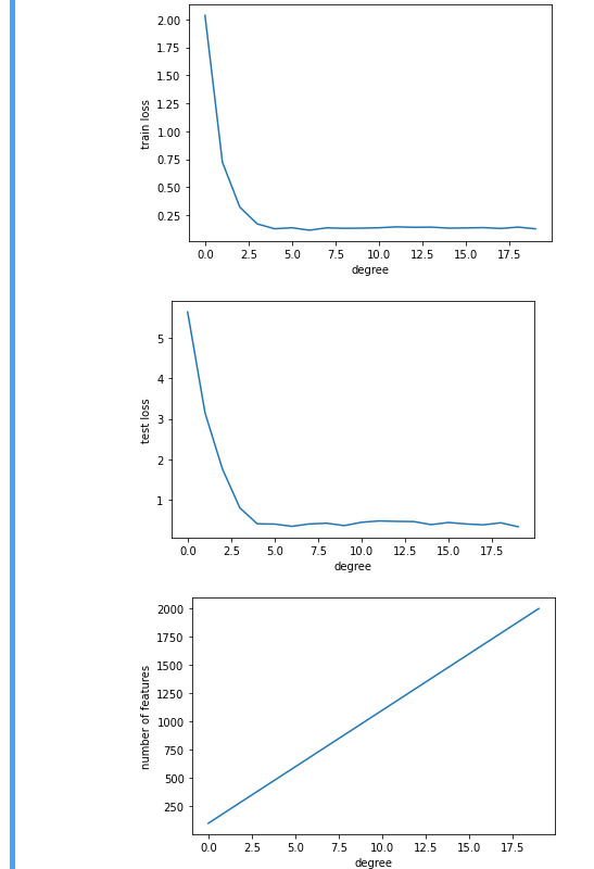
question 2: after 2 degrees, both reach nearly zero error
def train_2(train_features, test_features, train_labels, test_labels,
num_epochs=400):
loss = nn.MSELoss()
input_shape = train_features.shape[-1]
# Switch off the bias since we already catered for it in the polynomial
# features
net = nn.Sequential(nn.Linear(input_shape, 1, bias=False))
batch_size = min(10, train_labels.shape[0])
train_iter = d2l.load_array((train_features, train_labels.reshape(-1,1)),
batch_size)
test_iter = d2l.load_array((test_features, test_labels.reshape(-1,1)),
batch_size, is_train=False)
trainer = torch.optim.SGD(net.parameters(), lr=0.01)
for epoch in range(num_epochs):
    d2l.train_epoch_ch3(net, train_iter, loss, trainer)

return (evaluate_loss(net, train_iter, loss),
        evaluate_loss(net, test_iter, loss))
train_losses = []
test_losses = []
for i in range(1, len(poly_features[0]) + 1):
train_loss, test_loss = train_2(poly_features[:n_train, :i], poly_features[n_train:, :i], labels[:n_train], labels[n_train:])
train_losses.append(train_loss)
test_losses.append(test_loss)
bascially it is telling us the complexity will reduce the error and go to overfitting once beyond a point
Hi! In Section 4.4.3, under “Model complexity”, it reads “In fact, whenever the data examples each have a distinct value of x, a polynomial function with degree equal to the number of data examples can fit the training set perfectly.”. Although this is true, it could be a little misleading to the unaware reader, who might, for example, think that a second-degree polynomial is needed to perfectly fit two data points, whereas a linear function would suffice. Therefore, it could be more general to say that “[…] a polynomial function with degree d >= n - 1 can fit the training set perfectly, where n is the number of data examples.”.
Hello, when I try to solve the third question:
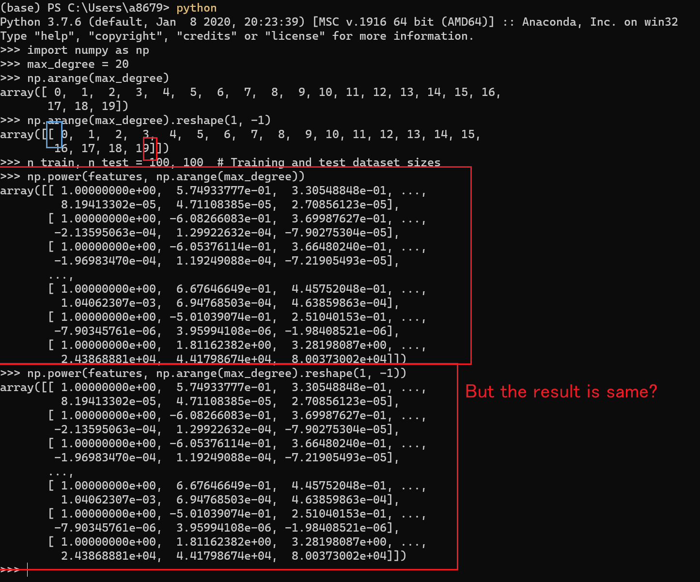
3. What happens if you drop the normalization (1/i!1/i!) of the polynomial features xixi? Can you fix this in some other way?
I found that I cannot get the answer when I increase the degree of the model to 6 or greater because of the explosion of gradient. I tried to fix it by decrease the learning ratio(1e-4) and increase the training epochs(1000) but got only little improvements (3.3 training error and 9.7 test error).
I wonder whether it is the right way to fix the problem or we have some other better solutions.
 Am I right?):