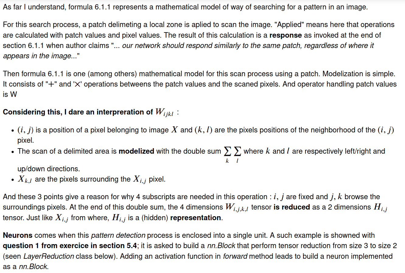
I may have an interpretation considering tensor dimensions.
There is a non evident connection with neurons, as explained at the end of the screenshot below.
yeah, i think we should know the underlying theories instead of the direct results.
from 6.1.1 we know that k,l are not relevant to i,j but in subsequent equation we know that a,b are as offsets to i,j. these mean that a,b now are relevant to i,j.
I think this is correct IFF the a,b are both from -infinite to infinite.
what is the real meaning about from W to V except subscripts? only for a rewriting as filter?
why is it necessary that for both X,H have same shape in 6.1.1?
I agree, in case of equivalence with MLP processing, then H is a representation of X with same shape (same area).
Re-writing 6.1.1 with introduction of subscripts (a,b), allows to consider sums with bounds. Those bounds depends of size of a and b as shown in 6.1.3; then (a,b) both can be regarded as distances around (i,j) and they can now be interpreted as geometric limits, say, a neighborhood of (i,j).
Due to area calculation restriction, “filter” term can now take place.
And as the section title claims, “Constraining MLP”, same calculations then MLP take place but on an arbitrary restricted area.
On my point of view, if calculations are restricted to a neighbourhood of (i,j), then W is no more equals to V. I think that if it is supposed that H and X have the same shape, after restriction of calculation to a neighbourhood of (i,j), it won’t be naymore the case.
sorry, i am not clear yet about the ‘same shape’ problem.
for instance ,an MLP with an image (10x10,ie. total 100 features) as input ,then the direct hidden layer is (4x4,ie. 16 units). how do you detailedly describe the ‘same shape’? does it only mean same spatial structure(ie. two dimensions) ?
in formula 6.1.1 ,it’s no doubt about the meaning of k,l(k=0,1,…9; l=0,1,…9) since each unit in hidden layer must sum over all input features with own weights,so k,l are not relevant to i,j(ie. public factors for hidden layer). but how about a,b now ?
thanks
I agree, for FC hidden layer, each unit has its own weights and, as fare I understand your purpose, then weights calculation leads to values that are independant from each pixels position indexed with (i,j).
But this is same when applying a translation transformation over subscripts with (a,b);
Reason is that when feeding 2D image into an MLP estimator, input layer is flattenered as a vector.
Browsing dimensions with (k,l) or (a,b) leads to same results for weights. Such representation leads to same weights calculation.
For shapes of input data and its representation from hidden layer :
when hidden layer has same number of nodes then pixels into input layer, then H, the representation of X into hidden layer, is regarded as having same dimension (same number of pixels) then X, input image.
When this number of units is less, H is regarded as a dimension reduction of input X
when number of units is greater then number of pixels from X, H is regarded as dimension projection in a greater space (analogy could be set with kernel trick).
I think that may be, the inroduction of (a,b) allows to introduce concept of neighbourhood and then, concept of feature map in which (k,l) becomes dependant (relevant) from (i,j) when weights are shared among each node from hidden layer.
The fourth dimension in eq 6.1.7 is batch size I guess. As the input tensors are of three dimention with height * width * channel. So to represent the equation with four variable it must be the batch size.
In formula 6.1.7, could we modify it to have bias term included? I have been confused about the index of bias term when multiple channels are involved in the convolutional layer.
Well I don’t think the forth dimension represents the batch size. The idea is that you can have multiple kernels applied to the same image and have multiple layers. So you have H x W x C (Height width channels) as input from the image than the output is a hidden layer that has D channels (this represents the number of kernels you apply to the image) So in the begging the channels are the colors RGB and afterwards you get a channel that might represent vertical edges horizontal edges corners etc. they get more abstract. The forth dimension in the case says how many abstract channels you get in the hidden layer.
PS Usually you don’t have a separate set of weights for each example in the batch. You are training one model.
Not sure if anyone uses this term.
So invariant means that something doesn’t change if some action is applied. So if you roll 5 dices the sum depends on the value of each die but not on the order in which they were rolled, so you might say the sum is order invariant. If you play a game where you win if your second roll is greater than the first this is no longer order invariant, so you might say it is order ‘variant’. I don’t think that anyone does that though.
A case when you might not want your network to the model to have translation invariance is in the setup of controlled environment where you have a prior knowledge of the expected structure of the image.
Assume that the size of the convolution kernel is Δ=0. Show that in this case the convolution kernel implements an MLP independently for each set of channels.
I can see how this is a MLP on pixel level but not on the channel level. In this case you can think of each pixel(all channels) as an example and the whole image as the batch. Please correct me if I’m wrong.
If we use Δ=0, then to calculate each H[i, j, :] only (i, j) pixel will be used. But the last dimension (new channels of H) will be computed as a H[i, j, d] = (Sum over all channels) V[0, 0, c, d] * X[i, j, c]. So basically you are computing a linear regression for each channel d using c channels of the (i, j) pixel. And because there may be multiple d channels, it is a linear layer. If we add following activation function and another layers we get an MLP.
This article is well written however I would like to point out an inconsistency with regards to the mathematics. There’s a difference between invariance and equivariance, and the meaning of both are used interchangeably in the article when they are most definitely not interchangeable.
Invariance means that for a function f:A->B and an action g, f(g.x) = f(x) for x in A. This means that whatever the input is to a function, if you apply an action g on it, the function f is invariant to the action g. With regards to the article, this would imply that translational invariance means translating an image won’t change anything to the hidden representation, by definition of invariance.
Equivariance (which I believe is the term you are looking for) means, with the above-defined f(g.x) = g.f(x). Therefore, acting on an input x by g, then applying f is the same as applying f on x and then acting by g. In the context of the article, translational equivariance is the idea that translating (g) the input x would result in a hidden activation of translating the hidden activation by that same translation.
A convolution, as defined in the article, would therefore be translationally equivariant, whilst something like local or max pooling would be locally or resp. globally invariant to permutations over its receptive field.
"Consequently, the number of parameters required is no longer 10^12 but a much more reasonable 4 ⋅ 10 ^6 ". could you please explain to me how it is 4 times 10^6 it should be 2 times only.
This threw me off to until I realised it’s an approximation, only exact in the limit Δ → ∞.
Consider the case Δ = 1, i.e. a and b both take values -1,0,1 so that V has 3*3=9 weights in total. This can also be written (2 Δ + 1)^2 = 4 Δ^2 + 4 Δ + 1 ≈ 4 Δ^2 when Δ is large.
For Δ=1 the approximation is pretty bad, 4 vs the true 9, but for Δ=1000 it’s not too bad: 4 million vs 4004001.