but i wonder know that why you add l2 on (o-y)? i think (o-y) is the derivative of ∂l/∂o while L2 is used in the bias whic like ||W||^2,so i think it’s a constant item .thanks
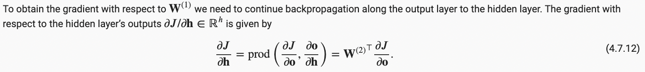
I can understand equation 4.7.12, as shown below, and the order of the elements in the matrix multiplication makes sense, i.e. the derivative of J w.r.t. h (gradient of h) is the product of the transpose of the derivative of o w.r.t. h (which is W2 in this case) and the derivative of J w.r.t. o (i.e. the gradient of o).
我可以理解等式 4.7.12, 也就是说,损失J对h的偏导数,也即h的梯度,等于h对于o的偏导数的转置与损失对于o的偏导数,也即o的梯度的乘积。
This is consistent with what Roger Grosse explained in his course that backprop is like passing error message, and the derivative of the loss w.r.t. a parent node/variable = SUM of the products between the transpose of the derivative of each of its child nodes/variables w.r.t. the parent (i.e. the transpose of the Jacobian matrix) and the derivative of the loss w.r.t. each of its children.
这与Roger Grosse的课程里对反向传播的解释是一致的,也就是说,反向传播是在传递误差信息,而损失对于当前父变量的导数,也即该父变量的梯度,等于所有其子变量对父变量的导数的转置,也即雅可比矩阵的转置与损失对于相应子变量的导数,也即子变量的梯度的乘积之总和。
However, this conceptual logic is not followed in equations 4.7.11 and 4.7.14 in which the “transpose” part is put after the “partial derivative part”, rather than in front of it. This could lead to problem in dimension mismatching for matrix multiplication in code implementation.
但似乎这一概念逻辑在等式 4.7.11和4.7.14中并没有被遵从,其中的雅可比矩阵转置的部分被放在了损失对子变量的导数的后面。这会导致在矩阵乘积运算中维度不匹配的问题。
Could the authors kindly explain if this is a typo, or the order in matrix multiplication as shown in the equations doesn’t matter because it is only “illustrative”? Thanks.
所以,可否请作者们解释一下,这是否是文字排版错误,抑或这个“顺序”在这些作为概念演示的等式里并不重要? 谢谢。
2 Likes
Exercises and my silly answers
- Assume that the inputs X to some scalar function f are n × m matrices. What is the dimensionality of the gradient of f with respect to X?
- Dimensionality reamains the same I tried be look at X.grad values.
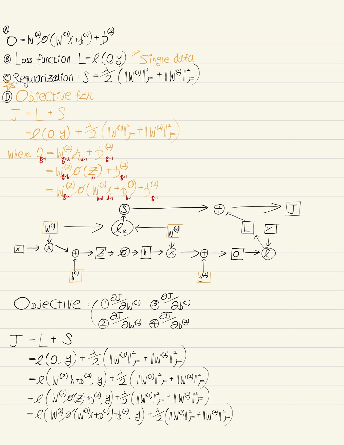
- Add a bias to the hidden layer of the model described in this section (you do not need to
include bias in the regularization term).
-
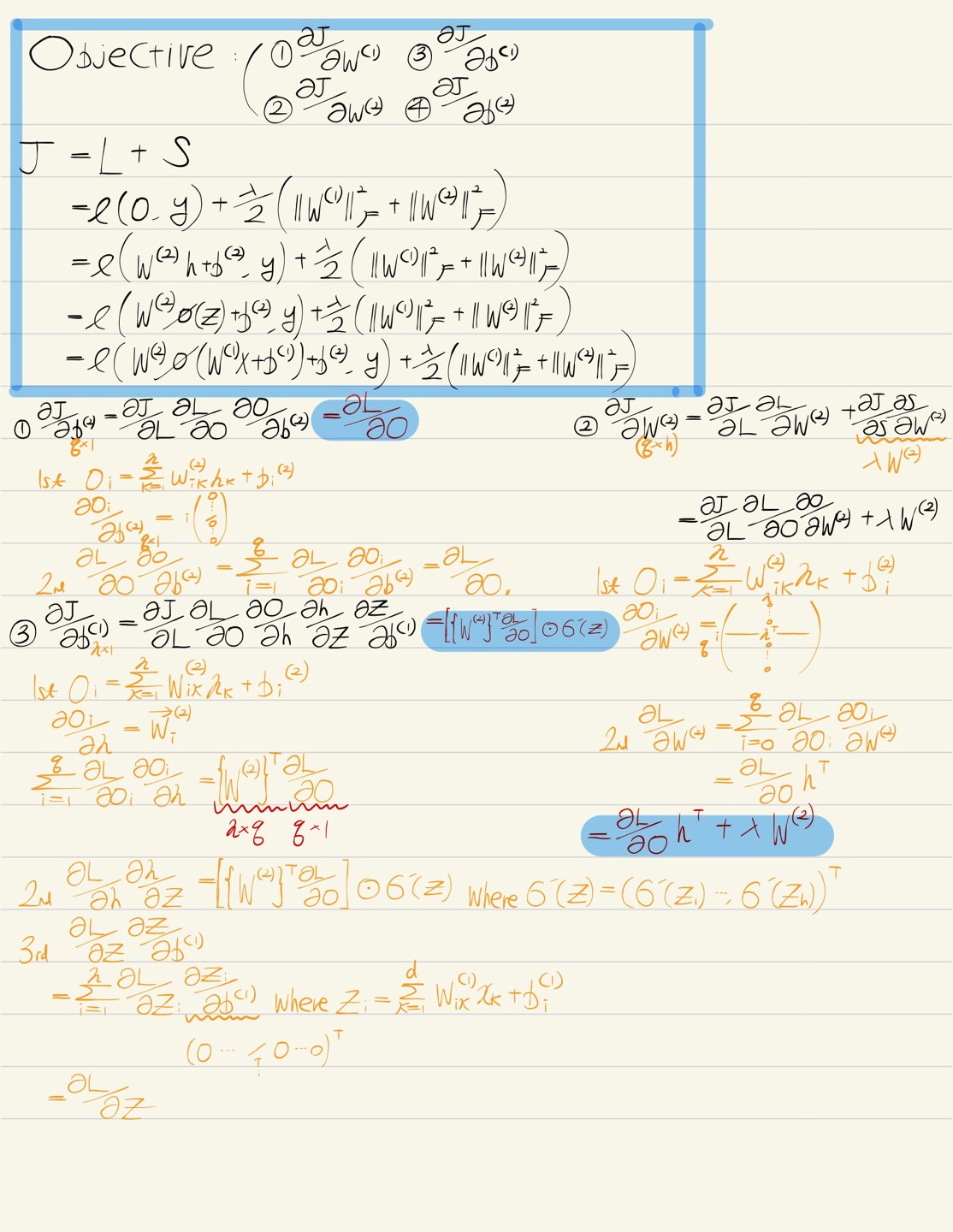
Draw the corresponding computational graph.
-
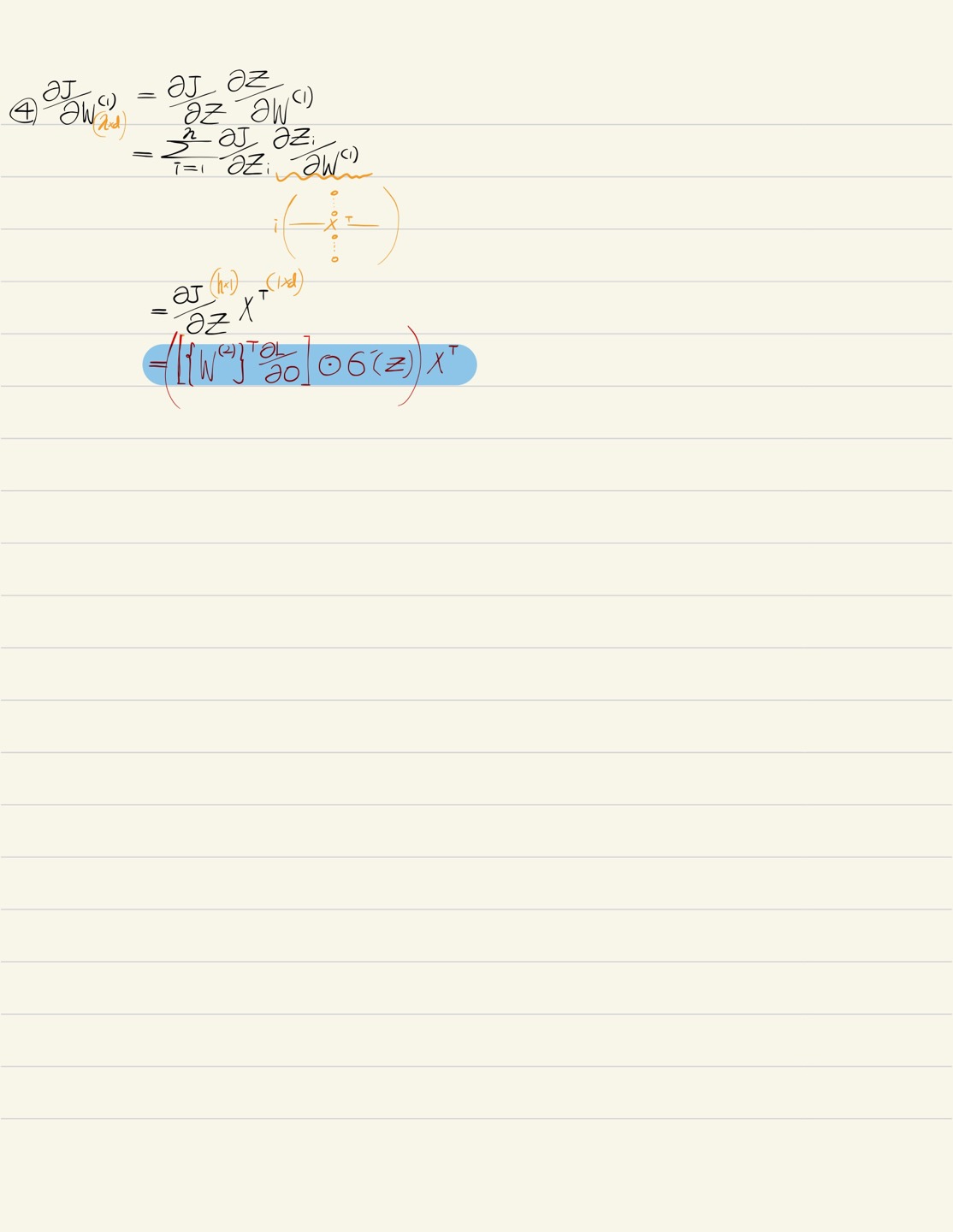
Derive the forward and backward propagation equations.
- given in the pic. There is almost no change.
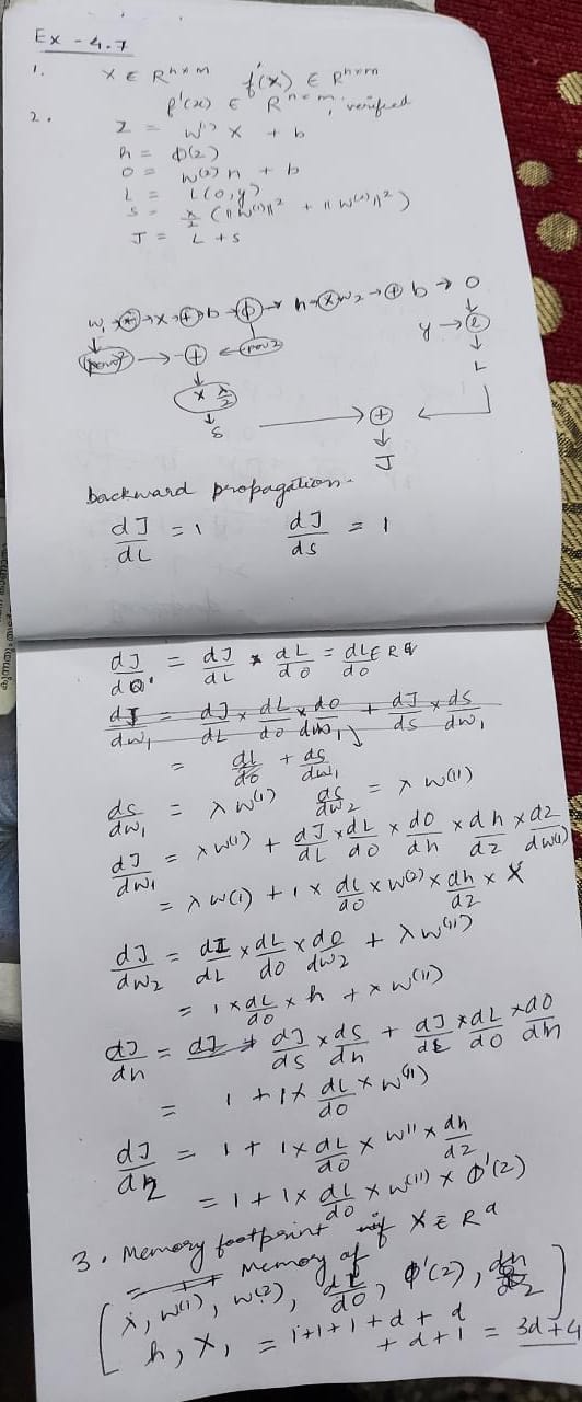
- Compute the memory footprint for training and prediction in the model described in this
section.
- If we are to assume that X belongs to R^d then , you would need to store dl/do, dh/dz, X, lambda, W(1), W(2), h, X.grad so considering X size is d then 4d + 4. Based on gradients calculated above. Rest all can be derived.
- Assume that you want to compute second derivatives. What happens to the computational
graph? How long do you expect the calculation to take?
- dont know how to come up with a solution to this
-
Assume that the computational graph is too large for your GPU.
- Can you partition it over more than one GPU?
- maybe computational grapha can be devided but there needs to be tmiing pipeline else one part would wait for the other. Maybe different batchwise the multiple GPU can be recruited.
- What are the advantages and disadvantages over training on a smaller minibatch?
- smaller minibatch takes more time and less memory and vice versa. Its a time space tradeoff.
I cannot answer your question but I am in awe how rigorously you have asked your question!
As far as I can see the notation - do / dW(2) in (4.7.11) is a vector-by-matrix derivative. Where can I read about how do you interpret such a notation? The wikipedia article (" Matrix calculus") says “These are not as widely considered and a notation is not widely agreed upon.” in a paragraph “Other matrix derivatives”. Tried other sources, haven’t found anything.
1 Like
In exercise 4 there is mentioning of second derivatives. Curious what are some examples when we want to compute second derivatives in practice?
I’m late to this but I did the math and I think you are correct, the “transpose of h” should be put in front of the “partial derivative part”.
My exercise:
- n * m;
2.1 insert b^(1)->(+) between (x)->z; insert b^(2)->(+) between (x)->o;
2.2
forward: pass;
backward:
partial J/ partial W^(1) and p J / pl W^(2) remain the same;
p J / p b^(2) = p J / p o, p J / p b^(1) = p J / p z; - Forward: only need preserve the current variables;
backward: preserve almost all intermediate variables; - more complex computational graph? more time?
5.1 yes; communicate with mpi or other things like;
5.2 buy space with time.
If folks still confused take a look at