http://d2l.ai/chapter_convolutional-neural-networks/conv-layer.html
Hey @anirudh in section 6.2.4 Learning A Kernel
when printing this at the bottom of our for loop:
if (i+1) % 2 == 0:
print(f'batch {i+1}, loss {l.sum():.3f}')
should it be batch or epoch? I thought it was epoch, could you explain why its batch instead?
1 Like
- When you try to automatically find the gradient for the Conv2D class we created, what kind of error message do you see?
Got Error Message: Inplace operations are not supported using autograd .
- How do you represent a cross-correlation operation as a matrix multiplication by changing the input and kernel tensors?
–> flip the two-dimensional kernel tensor both horizontally and vertically, and then perform the cross-correlation operation with the input tensor
K = torch.tensor([[1.0, -1.0]]) # filter shape: (1, 2)
# flip horizontally
K = torch.flip(K, [1])
# flip vertically
K = torch.flip(K, [0])
print(K)
print(K)

 Y = corr2d(X, K)
 plt.imshow(Y, cmap="gray")
What is the minimum size of a kernel to obtain a derivative of degree d?
–> I have no idea about this. Can someone clarify?
1 Like
For Exercise 2, l.sum().backward() is already computing the gradient, is it not?
how did you automatically try to find gradient?
yes through backpropagation the leaf tensor gradient is stored in net.grad
Exercises
-
Construct an image X with diagonal edges.
-
What happens if you apply the kernel K in this section to it?
- zero matrix.
-
What happens if you transpose X?
- No change
-
What happens if you transpose K?
- zero matrix.
-
-
When you try to automatically find the gradient for the Conv2D class we created, what kind
of error message do you see?
* I am able to do `net.weights.grad`, when I try `net.grad` I get the error `'Conv2d' object has no attribute 'grad'`
- How do you represent a cross-correlation operation as a matrix multiplication by changing
the input and kernel tensors?
* cross correlation is basically matrix multiplication between slices of tensorfrom X of the shape of kernel and summing.

* It can be done by padding Kand X based on what is needed to multiply
-
Design some kernels manually.
-
What is the form of a kernel for the second derivative?
- okay in order to compute one way would be to manually compute the second derivative and then let see a kernel be made using backpropogation
https://dsp.stackexchange.com/questions/10605/kernels-to-compute-second-order-derivative-of-digital-image
- okay in order to compute one way would be to manually compute the second derivative and then let see a kernel be made using backpropogation
-
What is the kernel for an integral?
- how do you actually make it manually
-
-
What is the minimum size of a kernel to obtain a derivative of degree d
* dont know.
I think so,epoch is batter than batch.
Construct an image X with diagonal edges.
-
What happens if you apply the kernel
Kin this section to it?
it detects the diagonal edges -
What happens if you transpose
X?
same -
What happens if you transpose
K?
same also -
How do you represent a cross-correlation operation as a matrix multiplication by changing the input and kernel tensors?
transforming the kernal in a matrix
Km = torch.zeros((9,5))
kv = torch.tensor([0.0,1.0,0.0,2.0,3.0])
for i in range(4):
Km[i:i+5,i] = kv
Km = Km.t()
Km = Km[torch.arange(Km.size(0))!=2]
Km = Km.t()
Km = tensor([[0., 0., 0., 0.],
[1., 0., 0., 0.],
[0., 1., 0., 0.],
[2., 0., 0., 0.],
[3., 2., 1., 0.],
[0., 3., 0., 0.],
[0., 0., 2., 0.],
[0., 0., 3., 0.],
[0., 0., 0., 0.]])
transforming the input X in a vector
X = torch.tensor([[float(i) for i in range(9)]])
X = tensor([[0., 1., 2., 3., 4., 5., 6., 7., 8.]])
X @ Km #matrix multiplication
result : tensor([[19., 25., 37., 0.]])
We reprint a key figure in Fig. 7.2.2 to illustrate the striking similarities.
What similarities is Fig. 7.2.2 trying to illustrate? I mean, what is being compared to what?
following this

After all, for a function $$f(i,j)$ its derivative $-\partial_i f(i,j) = \lim_{\epsilon \to 0} \frac{f(i,j) - f(i+\epsilon,j)}{\epsilon}$$
I got difference operator for the second derivative is [-1, 0, -1]
CODE
X = torch.ones((6, 8))
X[:, 2:6] = 0
K = torch.tensor([[1.0, -1.0]])
derivative1 = corr2d(X, K)
derivative2 = corr2d(derivative1, K)
print(derivative2)
@#OUT
tensor([[-1., 1., 0., 0., 1., -1.],
[-1., 1., 0., 0., 1., -1.],
[-1., 1., 0., 0., 1., -1.],
[-1., 1., 0., 0., 1., -1.],
[-1., 1., 0., 0., 1., -1.],
[-1., 1., 0., 0., 1., -1.]])
K = torch.tensor([[-1.0, 0.0, -1.0]])
derivative2 = corr2d(X, K)
print(derivative2)
@#OUT
tensor([[-1., -1., 0., 0., -1., -1.],
[-1., -1., 0., 0., -1., -1.],
[-1., -1., 0., 0., -1., -1.],
[-1., -1., 0., 0., -1., -1.],
[-1., -1., 0., 0., -1., -1.],
[-1., -1., 0., 0., -1., -1.]])
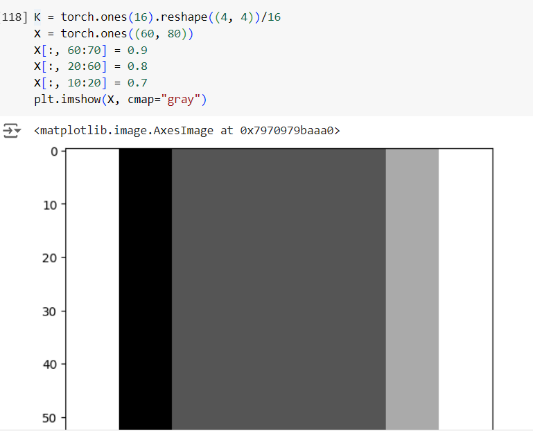
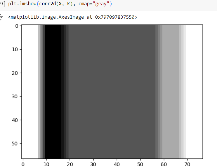
- How would you design a blur kernel? Why might you want to use such a kernel?
-
blur_deg = 4
-
K = torch.ones(blur_deg2).reshape((blur_deg, blur_deg))/blur_deg2
- What is the minimum size of a kernel to obtain a derivative of order $d$?
- d+1
Hi, thank you for the intuition on this. I can see different results but make sense that the second derivative is:
Y2 = corr2d( cordd2d ( X, K), K)
Applying this manually for the first tree elements of X I can see this:
kernel: 1.0, -1.0 | 1.0, -1.0
X[0, :3] = 110
naming elements:
a, b, c = X[0, 0], X[0, 1], X[0, 2]

the first derivative reduces the expresion to two elements
e, f = a - b, b - c
similarly the second rerivative generates one final element
g = e - f = (a - b ) - (b - c) = a -2b + c

hence the kernel will be [1, -2, 1]
Code:
X = torch.ones((1, 8))
X[:, 2:6] = 0
K = torch.tensor([[1.0, -1.0]])
Y = corr2d(corr2d(X, K), K)
Y
tensor([[-1.,  1.,  0.,  0.,  1., -1.]])
KK = torch.tensor([[1.0, -2.0, 1.0]])
YY = corr2d(X, KK)
YY
tensor([[-1.,  1.,  0.,  0.,  1., -1.]])
Exercise 2.1:
Say we have a function f(x, y) for an Image I, at any given coordinates x, y, it gives us the the color of the (x, y) pixel in I.
We can take the derivative of f with respect to x or y. If there is no edge at a point, that means all the other nearby points have the same color,
so the derivative at that point is zero.
If df/dx is non-zero, that means, there’s an age, in the direction of y. For example take this image:
1 1 1 0 0
1 1 1 0 0
1 1 1 0 0
There is a vertical edge here. df/dx at (x=3, y=0,1,2) is non-zero. When you move along the direction of the edge(y) there is no change in the pixel values.
When you move perpendicular to the direction of the edge(x), the pixel values change(and the derivative is nonzero).
Now to take the derivative in any direction, we simply have to calculate the dot product of the gradient and the directional vector.
So to detect edges along (-v2, v1), we need to find the derivative along the direction of the (v1, v2) vector.
Meaning: (v1, v2) * (df/dx, df/dy)
Now since in our case, f is usually a discrete function, we have to calculate the derivative with a finite difference approximation(e.g f(x+1) - f(x))
df/dx =

[[  1, -1],
 [  1, -1]]
df/dy =

[[  1,  1],
 [ -1, -1]]
so we have:
v1 * df/dx + v2 * df/dy =

[[  v1 + v2, -v1 + v2],
 [  v1 - v2, -v1 - v2]]
This is a crude edge-detector since it can only detect edges along the directions (0, 1), (1, 0), (1, 1) & (1, -1)
To increase the persicion in the direction, we can use larger kernels:
v1
*
[[ 1, 0, -1],
 [ 1, 0, -1],
 [ 1, 0, -1]]

+

v2
*
[[ 1,  1,  1],
 [ 0,  0,  0],
 [-1, -1, -1]]
Exercise 2.2:
First order derivative at x:
f(x+1) - f(x)
With that definition the second order derivative at x becomes:
f'(x+1) - f'(x)
Replace f’ with its the first order formula above:
(f(x+2) - f(x+1)) - (f(x+1) - f(x))
We get:
f(x+2) - 2 * f(x+1) + f(x)
Write it as a vector:
[1, -2, 1]
The minimum size of such a kernel is 1x3 or 3x1
It doesn’t respond to constant areas where all pixel values are the same.
It responds to thin lines, sole pixels, or edges as usual. It doesn’t respond to linear increase in the pixels: 0, 1, 2, 3, 4, 5 or 0, 2, 4, 6, 8, 10 because the derivative is constant([1, 1, 1, 1] or [2, 2, 2, 2])
A simple average can make a blur kernel:
[[1/4, 1/4],
[1/4, 1/4]]
This gets rid of the noisy thin lines or sole pixel that the [1, -2, 1] vector responds to strongly. It could make edge detection work better by getting rid of those fake edges. We could also create larger kernels that use Gaussian-like distributions in the weights of the matrix, giving more weight to the pixels closer to the center and less weight to the weights further away.
2 points gives us one derivative(f’(x)). 3 points gives us 2 derivatives(f’(x+1), f’(x)). 4 points gives us 3 derivatives(f’(x+2), f’(x+1), f’(x))
Say we have n points. We get n-1 first order derivatives. Thus we get n-2 second order derivatives. n-3 third order derivatives. Keep going, until n - (n-1) : 1. So for an (n-1) order derivative, we need n points. Meaning, for a d order derivative, we need d+1 points.
Exercise 4:
Say we have a 2 by 2 kernel, and a 3 by 3 image. These are the pixels(counting from 0 to 8) that the kernel would slide:
0, 1
3, 4

1, 2
4, 5

3, 4
6, 7

4, 5
7, 8
Flatten each of these into a row (or column) vector, and stack the rows (or columns) together to make a matrix.
[[0, 1, 2, 3],
 [1, 2, 4, 5],
 [3, 4, 6, 7],
 [4, 5, 7, 8]]
Now flatten the kernel into a column (or row) vector, and multiply the above matrix by that vector. It should give us the value for each of the four patches.