https://zh.d2l.ai/chapter_linear-networks/linear-regression.html
1 Like
中文版第二版纸质书啥时候出版呢? 
没有答案  题目有点难哈哈哈
这样对不对呢
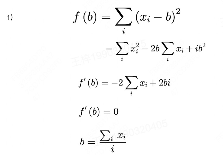
- 问题1:已知 𝑥1,…,𝑥𝑛∈ℝ,目标找到𝑏,使得最小化 ∑(𝑥𝑖−𝑏)^2
- 设 𝑦𝑖= 𝑥𝑖 - 𝑏,问题转化为Y = ∑𝑦𝑖^2,展开
- Y = ∑(𝑥𝑖^2 - 2𝑥𝑖·𝑏 + 𝑏^2) = ∑𝑥𝑖^2 - 2∑𝑥𝑖·𝑏 + n·𝑏^2
- 把 ∑𝑥𝑖^2 和 2∑𝑥𝑖视为常数,则转化为关于b的一元二次方程
- 由于n>0,有最小值,计算地𝑏解析解为:
1/n·∑𝑥𝑖 + 1/n·√((∑𝑥𝑖)^2 - n∑𝑥𝑖^2)) 或
1/n·∑𝑥𝑖 - 1/n·√((∑𝑥𝑖)^2 - n∑𝑥𝑖^2)) - 前提:√((∑𝑥𝑖)^2 - n∑𝑥𝑖^2)) ≥0
是不是应该用矩阵或向量的形式表述?
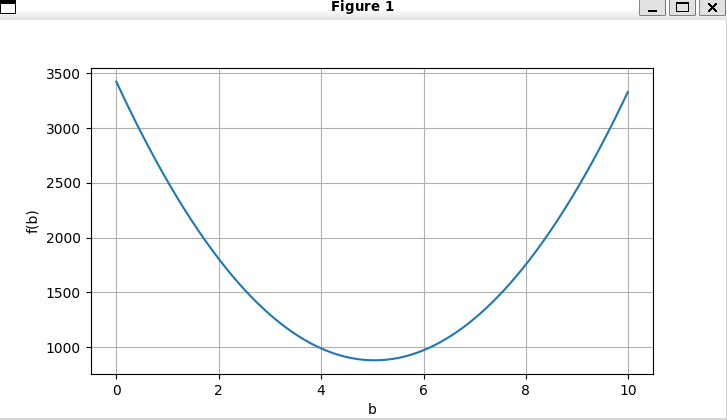
从含义上理解, 𝑥𝑖是直线上的一些点,使∑(𝑥𝑖−𝑏)^2最小,可以理解为到每个点的距离和最小,结果应该是所有点的均值所在的点
同问:假设我们有⼀些数据x1, . . . , xn ∈ R。我们的⽬标是找到⼀个常数b,使得最小化∑
i
(xi − b)
2。
这个应该怎么使用线性回归的方式去处理的,房屋价格问题我倒是一知半解的,程序员的逻辑思维还不能好好转变过来
请问From d2l import torch as d2l
最后报错SyntaxError: invalid syntax该怎么处理
F大写了?就这一句还能有语法错误呢,。。。。。。
###########################
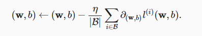

梯度下降公式里,是每个样本的loss对参数求导再求和。
但在程序中,是多个样本的loss之和再对参数求导 ???
第一题直接展开求导,得最小值,高中数学。
对于第一问,我的解法是设X的均值为 x* ;
∑(xi-b)^2 = ∑(xi - x* + t)^2 = ∑(xi - x*)^2 + 2t(xi - x*) + t^2
=∑(xi - x*)^2 + nt^2 + 0 (由于∑xi = nx,∑2t(xi - x*)值为0)
因此,当t = 0时,∑(xi-b)^2取得最小值为 D(X)。
故b = x*
至于与正态分布的关系,大概说的应该是中心极限定律。
3.1.6 练习题1
- 平方的求和是一个恒定大于等于0的式子,所以当曲线变化率接近0的时候我认为是一个最小值点,故求导并让导数值 = 0时,b等于x的均值。
- 说实话不是很明白,我想会不会是如果记x轴为x_i - b的差值区间, y轴为差值属于这个区间的元素数量,那么满足最优解的时候这张图我认为也应该要呈现出一种正太分布的样子
微分操作是线性的,所以先微分还是先求和没有区别
逻辑回归才是极大似然估计啊,这本书提到线性回归也是,是不是错了?
先执行 !pip install d2l 就可以了
#!/usr/bin/env python3

import numpy as np
import torch

class Linear:
    def __init__(self, n, eta=0.01):
        self.theta = torch.normal(0.0, 1.0, size=(n+1, 1), requires_grad=True)
        self.eta = eta

    def cal(self, x):
        return torch.concat((x, torch.ones(x.shape[0], 1)), dim=1) @ self.theta

    def loss(self, x, y):
        return (y - self.cal(x)) ** 2

    def batch(self, x, y):
        loss = self.loss(x, y).sum()
        loss.backward()
        with torch.no_grad():
            self.theta -= self.eta * self.theta.grad / x.shape[0]
            print(f'loss={loss};theta={self.theta.reshape(3)}')


def synthetic_data(w, b, num_examples):
    """生成y=Xw+b+噪声"""
    X = torch.normal(0.0, 1.0, (num_examples, len(w)))
    y = torch.matmul(X, w) + b
    y += torch.normal(0, 0.01, y.shape)
    return X, y.reshape((-1, 1))

true_w = torch.tensor([2, -3.4])
true_b = 4.2
features, labels = synthetic_data(true_w, true_b, 10)
mod = Linear(2)
for i in range(100):
    x, y = synthetic_data(true_w, true_b, 10)
    mod.batch(x, y)
我尝试理解之后自己写了一个线性层,但是不同的随机数据集训练出的结果差别非常大,有没有哪位大哥帮我看看是不是有什么问题?
结果如下:
loss=531.988525390625;theta=tensor([ 0.6741,  1.5314, -1.5466], requires_grad=True)
loss=519.7105102539062;theta=tensor([ 0.6976,  1.3687, -1.3290], requires_grad=True)
loss=860.7129516601562;theta=tensor([ 0.8107,  1.0294, -0.9735], requires_grad=True)
loss=505.11395263671875;theta=tensor([ 0.9274,  0.5874, -0.5116], requires_grad=True)
loss=494.73187255859375;theta=tensor([ 1.0005, -0.0031,  0.0446], requires_grad=True)
loss=119.57245635986328;theta=tensor([ 1.0954, -0.5914,  0.6550], requires_grad=True)
loss=430.96051025390625;theta=tensor([ 1.2534, -1.3290,  1.3740], requires_grad=True)
loss=123.87307739257812;theta=tensor([ 1.4306, -2.1071,  2.1459], requires_grad=True)
loss=51.164485931396484;theta=tensor([ 1.6061, -2.9124,  2.9511], requires_grad=True)
loss=15.387931823730469;theta=tensor([ 1.7819, -3.7230,  3.7787], requires_grad=True)
loss=3.40395188331604;theta=tensor([ 1.9626, -4.5278,  4.6152], requires_grad=True)
loss=9.35221004486084;theta=tensor([ 2.1452, -5.3155,  5.4533], requires_grad=True)
loss=33.502891540527344;theta=tensor([ 2.3234, -6.0670,  6.2937], requires_grad=True)
loss=81.21678924560547;theta=tensor([ 2.4986, -6.7785,  7.1082], requires_grad=True)
loss=233.32803344726562;theta=tensor([ 2.6764, -7.3922,  7.8752], requires_grad=True)
loss=233.37728881835938;theta=tensor([ 2.8734, -7.9556,  8.5663], requires_grad=True)
loss=369.426513671875;theta=tensor([ 3.0623, -8.3969,  9.2173], requires_grad=True)
loss=420.9701232910156;theta=tensor([ 3.2856, -8.7715,  9.7596], requires_grad=True)
loss=601.8832397460938;theta=tensor([ 3.5031, -9.0670, 10.1633], requires_grad=True)
loss=554.967529296875;theta=tensor([ 3.7319, -9.2916, 10.4454], requires_grad=True)
loss=1030.767333984375;theta=tensor([ 3.9408, -9.3487, 10.5607], requires_grad=True)
loss=229.73336791992188;theta=tensor([ 4.1317, -9.3879, 10.6261], requires_grad=True)
loss=1085.172119140625;theta=tensor([ 4.2593, -9.2684, 10.5228], requires_grad=True)
loss=386.8089599609375;theta=tensor([ 4.3602, -9.1315, 10.3227], requires_grad=True)
loss=811.8597412109375;theta=tensor([ 4.3966, -8.8539, 10.0138], requires_grad=True)
loss=1223.5562744140625;theta=tensor([ 4.3963, -8.3375,  9.5231], requires_grad=True)
loss=678.25732421875;theta=tensor([ 4.3390, -7.7299,  8.8878], requires_grad=True)
loss=620.6932983398438;theta=tensor([ 4.2797, -6.9790,  8.1211], requires_grad=True)
loss=182.00277709960938;theta=tensor([ 4.1823, -6.1867,  7.3215], requires_grad=True)
loss=226.32501220703125;theta=tensor([ 4.0558, -5.3382,  6.4473], requires_grad=True)
loss=134.9973602294922;theta=tensor([ 3.8888, -4.4538,  5.5208], requires_grad=True)
loss=68.11566162109375;theta=tensor([ 3.6709, -3.5516,  4.5785], requires_grad=True)
loss=38.36671447753906;theta=tensor([ 3.4085, -2.6362,  3.6344], requires_grad=True)
loss=12.295902252197266;theta=tensor([ 3.1286, -1.7215,  2.6891], requires_grad=True)
loss=123.59443664550781;theta=tensor([ 2.8058, -0.8948,  1.7775], requires_grad=True)
loss=144.82211303710938;theta=tensor([ 2.4594, -0.1241,  0.9196], requires_grad=True)
loss=197.0822296142578;theta=tensor([2.1257, 0.6030, 0.1401], requires_grad=True)
loss=454.7916259765625;theta=tensor([ 1.7994,  1.2222, -0.5215], requires_grad=True)
loss=672.1536254882812;theta=tensor([ 1.4390,  1.6701, -1.0648], requires_grad=True)
loss=402.4933776855469;theta=tensor([ 1.1109,  2.0062, -1.5661], requires_grad=True)
loss=784.4359741210938;theta=tensor([ 0.8341,  2.2291, -1.9096], requires_grad=True)
loss=326.7474060058594;theta=tensor([ 0.5518,  2.4344, -2.1612], requires_grad=True)
loss=656.53662109375;theta=tensor([ 0.2400,  2.4741, -2.3516], requires_grad=True)
loss=1191.728271484375;theta=tensor([-0.1010,  2.3200, -2.3443], requires_grad=True)
loss=474.1963195800781;theta=tensor([-0.4540,  2.1167, -2.2311], requires_grad=True)
loss=1050.075927734375;theta=tensor([-0.7888,  1.7115, -1.9715], requires_grad=True)
loss=882.9622192382812;theta=tensor([-1.0361,  1.1817, -1.5684], requires_grad=True)
loss=524.0263061523438;theta=tensor([-1.2242,  0.5748, -1.0761], requires_grad=True)
loss=347.0560302734375;theta=tensor([-1.3641, -0.0977, -0.5314], requires_grad=True)
loss=330.15216064453125;theta=tensor([-1.5000, -0.8499,  0.0946], requires_grad=True)
loss=227.52728271484375;theta=tensor([-1.6143, -1.6489,  0.7838], requires_grad=True)
loss=235.7517547607422;theta=tensor([-1.6353, -2.4838,  1.4942], requires_grad=True)
loss=200.72230529785156;theta=tensor([-1.5985, -3.3616,  2.2604], requires_grad=True)
loss=227.18133544921875;theta=tensor([-1.4603, -4.2472,  3.0725], requires_grad=True)
loss=145.7969512939453;theta=tensor([-1.2475, -5.1074,  3.8953], requires_grad=True)
loss=103.00408172607422;theta=tensor([-0.9966, -5.9170,  4.7048], requires_grad=True)
loss=245.4693603515625;theta=tensor([-0.6626, -6.6339,  5.4978], requires_grad=True)
loss=265.03265380859375;theta=tensor([-0.2661, -7.2382,  6.2913], requires_grad=True)
loss=233.37060546875;theta=tensor([ 0.1829, -7.7771,  7.0385], requires_grad=True)
loss=315.7805480957031;theta=tensor([ 0.7009, -8.2558,  7.7002], requires_grad=True)
loss=645.592529296875;theta=tensor([ 1.2346, -8.5653,  8.2334], requires_grad=True)
loss=145.95962524414062;theta=tensor([ 1.7392, -8.8296,  8.7464], requires_grad=True)
loss=331.44921875;theta=tensor([ 2.2040, -9.0297,  9.1879], requires_grad=True)
loss=942.5620727539062;theta=tensor([ 2.5506, -8.9755,  9.5437], requires_grad=True)
loss=467.2809753417969;theta=tensor([ 2.9046, -8.8704,  9.7770], requires_grad=True)
loss=478.8691101074219;theta=tensor([ 3.3476, -8.6963,  9.8919], requires_grad=True)
loss=850.0372924804688;theta=tensor([ 3.7364, -8.3141,  9.9146], requires_grad=True)
loss=608.9434814453125;theta=tensor([ 4.0938, -7.8360,  9.8162], requires_grad=True)
loss=647.3972778320312;theta=tensor([ 4.3668, -7.2417,  9.6103], requires_grad=True)
loss=211.79762268066406;theta=tensor([ 4.6553, -6.6351,  9.3280], requires_grad=True)
loss=167.3760223388672;theta=tensor([ 4.9267, -6.0448,  8.9791], requires_grad=True)
loss=264.1585388183594;theta=tensor([ 5.1460, -5.4350,  8.5622], requires_grad=True)
loss=265.04119873046875;theta=tensor([ 5.3491, -4.7818,  8.0559], requires_grad=True)
loss=227.40081787109375;theta=tensor([ 5.5051, -4.0909,  7.4859], requires_grad=True)
loss=292.4118957519531;theta=tensor([ 5.5879, -3.3750,  6.8214], requires_grad=True)
loss=226.05003356933594;theta=tensor([ 5.5892, -2.7248,  6.0967], requires_grad=True)
loss=249.56619262695312;theta=tensor([ 5.4731, -2.0723,  5.3298], requires_grad=True)
loss=152.64756774902344;theta=tensor([ 5.2790, -1.4308,  4.5453], requires_grad=True)
loss=285.6107177734375;theta=tensor([ 4.9527, -0.8647,  3.7928], requires_grad=True)
loss=122.79955291748047;theta=tensor([ 4.5621, -0.3228,  3.0252], requires_grad=True)
loss=121.6588363647461;theta=tensor([4.1250, 0.1900, 2.2874], requires_grad=True)
loss=275.0060729980469;theta=tensor([3.6451, 0.6170, 1.6285], requires_grad=True)
loss=233.96275329589844;theta=tensor([3.1393, 0.9647, 1.0111], requires_grad=True)
loss=386.85406494140625;theta=tensor([2.5418, 1.2107, 0.4645], requires_grad=True)
loss=543.2579956054688;theta=tensor([1.8463, 1.3148, 0.0193], requires_grad=True)
loss=225.1168975830078;theta=tensor([ 1.1082,  1.3510, -0.3929], requires_grad=True)
loss=632.675048828125;theta=tensor([ 0.3948,  1.2323, -0.6947], requires_grad=True)
loss=517.4296264648438;theta=tensor([-0.2903,  0.9903, -0.9111], requires_grad=True)
loss=506.6915283203125;theta=tensor([-0.8938,  0.6999, -1.0073], requires_grad=True)
loss=733.8193969726562;theta=tensor([-1.4347,  0.2982, -0.9444], requires_grad=True)
loss=292.29241943359375;theta=tensor([-1.9209, -0.0920, -0.7960], requires_grad=True)
loss=283.09063720703125;theta=tensor([-2.3847, -0.5569, -0.6015], requires_grad=True)
loss=567.23388671875;theta=tensor([-2.8089, -1.1203, -0.2652], requires_grad=True)
loss=229.3523406982422;theta=tensor([-3.1847, -1.6750,  0.1263], requires_grad=True)
loss=452.8999328613281;theta=tensor([-3.4409, -2.3028,  0.5568], requires_grad=True)
loss=262.04522705078125;theta=tensor([-3.6271, -2.8785,  1.0422], requires_grad=True)
loss=304.97216796875;theta=tensor([-3.7350, -3.4740,  1.5778], requires_grad=True)
loss=386.376220703125;theta=tensor([-3.7450, -4.0822,  2.1946], requires_grad=True)
loss=290.7869567871094;theta=tensor([-3.6587, -4.6811,  2.8225], requires_grad=True)
loss=281.5928039550781;theta=tensor([-3.4840, -5.2947,  3.5097], requires_grad=True)
3.1.11处这样描述,因此,我们现在可以写出通过给定的x观测到特定y的似然 (likelihood):
不应该是,我们根据给定的x和y 观测到噪声参数w和b取值的最大可信度吗?
为什么通常假设噪声符合正态分布?是默认做法还是有什么其它直觉上的考虑吗?
同意這個結果,我寫了一段程序得到的結果和這個相同。
import numpy as np
import torch
from d2l import torch as d2l

n = 100
x = np.random.uniform(0,10,n)

def f(b, x):
    y = x-b
    y *= y
    return y.sum()

b_range = np.arange(0, 10, 0.01)
b_values = []
for b in b_range:
    b_values.append(f(b,x))
min_b = np.min(b_values)
min_idx = np.where(b_values == min_b)[0]
print(f'{min_b} , {min_idx/100}, {np.mean(x):.2f}')
d2l.plot(b_range,[b_values],xlabel='b',ylabel='f(b)')
d2l.plt.show()
Strictly speaking, (3.1.1) is an affine transformation of input features, which is characterized by a linear transformation of features via a weighted sum, combined with a translation via the added bias.
这句话的中文翻译让人看起来有点费解,想表达的应该是:线性假设(加权求和的公式)是对输入特征的仿射变换,如果不考虑偏置,就是一个线性变换。(线性变换是一种特殊的仿射变换,其区别在于线性变换具有齐次性,而仿射变换满足非齐次性)