Linear Regression Implementation from Scratch

It computes the gradient of the tensor l.sum() with respect to w and b. Here is the documentation for this method.

The change is in the gradients, which are stored at the “free variables” w and b with respect to which the gradients are computed. You can retrieve these gradients, and see that they indeed change before and after a call to backward(), by inspecting the grad attribute of these variables, like so: w.grad , b.grad .

Why do we need param.grad.zero_() in sgd function?

In the function sgd(params, lr, batch_size) this line baffles me:

param -= lr * param.grad / batch_size

How is it possible for this line to update the external scope variable “w”? I did some testing and found the below behavior. Why does the first example update “z” whereas the second does not. Are scope rules different for PyTorch tensors?

Screen Shot 2022-01-04 at 3.48.34 AM

1 Like

function always fail d2l.plt.scatter(...), could you please help?

My solution about Exercise 2:

in thedata_iter, why batch_indices has to be converted to torch.tensor? a list also works, is there any particular consideration?

In section 3.4.4, we added a fit_epoch function to the Trainer class (copied below).

@d2l.add_to_class(d2l.Trainer)  #@save
def fit_epoch(self):
    self.model.train()
    for batch in self.train_dataloader:
        loss = self.model.training_step(self.prepare_batch(batch))
        self.optim.zero_grad()
        with torch.no_grad():  # why we use torch.no_grad() here??
            loss.backward()
            if self.gradient_clip_val > 0:
                self.clip_gradients(self.gradient_clip_val, self.model)
            self.optim.step()
        self.train_batch_idx += 1
    if self.val_dataloader is None:
        return
    self.model.eval()
    for batch in self.val_dataloader:
        with torch.no_grad():
            self.model.validation_step(self.prepare_batch(batch))
        self.val_batch_idx += 1

Inside the training loop (for batch in self.train_dataloader: …), why we enable the torch.no_grad() context manager?

According to pytorch’s doc: torch.no_grad() is a context-manager that disabled gradient calculation.

Disabling gradient calculation is useful for inference, when you are sure that you will not call Tensor.backward(). It will reduce memory consumption for computations that would otherwise have requires_grad=True.

However, we need to explicitly call loss.backward() within the training loop.

1 Like

My opinions for the exs:

I’ m not so sure about ex.7and ex.9 can anybody help me?

ex.1
1.Initialize the w to zeros.
2
2. Initialize w by norm distribution.
canvas
3. Initialize the w by norm distribution with sigma set to 1000
3

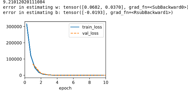
Note that I set max epoch to 10, seems like if I start w with all zero, it doesn’t make any difference, but if I change the sigma from 0.01 to 1000, the training speed doesn’t change, but the training error start with a huge quantity, and ends with a number increase by two orders of magnitude for both w and b.

ex.2
Step1 I produce a class to generate the examples composed by self.V = voltage, self.I = current, self.IR = I*R

%matplotlib inline
import torch
from d2l import torch as d2l
import random
class SyntheticRegressionData_202209031839(d2l.DataModule):
    def __init__(self, r_list, noise=0.1, num_train=100, num_val=100, batch_size=32, shuffle=True):
        super().__init__()
        self.save_hyperparameters()
        
        #for every resistor r, send some voltage and get some current
        #assume that the voltage is the range(1,num_train+1,1)
        V_train = torch.tensor([])
        V_val = torch.tensor([])
        I_train = torch.tensor([])
        I_val = torch.tensor([])
        IR_train = torch.tensor([])# to save the value of I*R
        IR_val = torch.tensor([])
        for r in r_list:
            #V_train_tmp=torch.abs(torch.randn(num_train, 1))
            V_train_tmp = torch.tensor(range(1,num_train+1,1)).reshape(-1,1)
            V_train = torch.cat((V_train, V_train_tmp), 0)
            I_train_tmp = V_train_tmp/r + torch.randn(num_train, 1) * noise
            I_train = torch.cat((I_train, I_train_tmp), 0)
            IR_train = torch.cat((IR_train, I_train_tmp*r), 0)
        for r in r_list:
            V_val_tmp = torch.tensor(range(1,num_val+1,1)).reshape(-1,1)
            V_val = torch.cat((V_val, V_val_tmp), 0)
            I_val_tmp = V_val_tmp/r + torch.randn(num_val, 1) * noise
            I_val = torch.cat((I_val, I_val_tmp), 0)
            IR_val = torch.cat((IR_val, I_val_tmp*r), 0)
        
        #need to be suffle or the examples will be ordered by the r value
        indices_train = list(range(0, self.num_train*len(r_list)))        
        indices_val = list(range(0, self.num_train*len(r_list)))
        if shuffle:
            random.shuffle(indices_train)
            random.shuffle(indices_val)      
        
        #combine examples for training and validating
        self.V = torch.cat((V_train[indices_train], V_val[indices_val]), 0)
        self.I = torch.cat((I_train[indices_train], I_val[indices_val]), 0)
        self.IR = torch.cat((IR_train[indices_train], IR_val[indices_val]), 0)

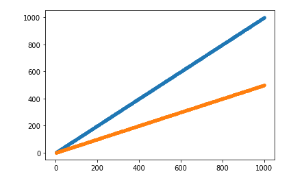
Step2 As I experimented with 2 different resistors, each one will be put voltage(I) vary from 1 to 100, and I evaluate the current(I), and plot them, judging from the image, the relation between I and V of the same resistor is linear.

import matplotlib.pyplot as plt
data_1= SyntheticRegressionData_202209031839([1])
data_2= SyntheticRegressionData_202209031839([2])
plt.plot(data_1.V, data_1.I, 'o', data_2.V, data_2.I, 'o')

5
Step3 Define the data loader.

@d2l.add_to_class(SyntheticRegressionData_202209031839)
def get_dataloader(self, train):
    #the real num_train is num_train*len(self.r_list)
    i = slice(0, self.num_train) if train else slice(self.num_train, None)
    return self.get_tensorloader((self.IR, self.V), train, i)

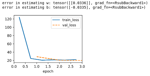
Step4 Train the model, learning rate is suggested to set to a small value, or it will get many NAN at the forward phase, and the conclution is that U = I*R.

data= SyntheticRegressionData_202209031839(r_list = range(1,11,1))
model = LinearRegressionScratch(1, lr=0.0003, sigma = 0.01)
trainer = d2l.Trainer(max_epochs=3)
trainer.fit(model, data)
print(f'error in estimating w: {1. - model.w}')
print(f'error in estimating b: {0. - model.b}')

6

ex.3
1
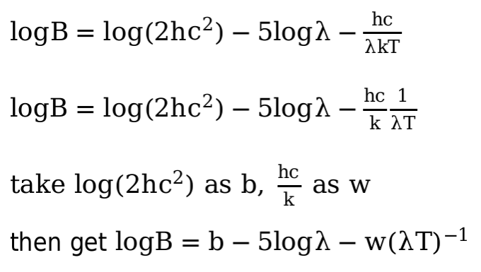
As the procedure shown in the picture, I think during the experiment, the λ, B, T can be preprocessed as logB, -5logλ, (λT)^-1, where logB will be the y, -5logλ and (λT)^-1 will be x1 and x2. Then the problem become a linear regression, after we have train out the w and b, we can use it to compute T with a B and λ.

ex.4
I tested with a simple linear function.

def loss(y_hat, y):
    l = (y_hat - y.reshape(y_hat.shape)) ** 2 / 2
    return l.mean()

x = torch.tensor([[1.,2.],[3.,4.]])
b = torch.tensor([1.]).requires_grad_(True)
w = torch.tensor([1.,2.]).reshape(-1,1).requires_grad_(True)
y_hat = (torch.matmul(x, w) + b)
y = torch.tensor([5.,6.])
loss = loss(y_hat, y)
loss.backward()
print(w.grad, b.grad)
loss.backward()
print(w.grad, b.grad)

The first backward works well , and the grad is tensor([[ 9.5000], [13.0000]]) tensor([3.5000])
But the second backward one cause a error:

RuntimeError: Trying to backward through the graph a second time (or directly access saved tensors after they have already been freed). Saved intermediate values of the graph are freed when you call .backward() or autograd.grad(). Specify retain_graph=True if you need to backward through the graph a second time or if you need to access saved tensors after calling backward.

As the ouput say, I should add “retain_graph=True” at the first backward() or the grad will be drop each automatically. So I change the code at the first backward to

loss.backward(retain_graph=True)

and the output is:
tensor([[ 9.5000], [13.0000]]) tensor([3.5000])
tensor([[19.], [26.]]) tensor([7.])
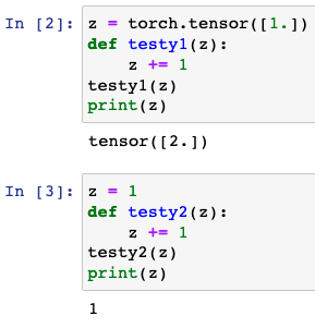
ex.5
I think because the element-wise subtraction can only be used between two tensors with same shape, unless one of them is a scalar.

ex.6
I use the same synthetic data in this chapter, test lr = [0.003, 0.03, 0.3, 3] with max_epoch = 3, and find that 0.03 is too small that the reducing of error(both train and val) is too slow, 3 is too large that the error keep growing as the epoch proceed, 0.3 is the fast one that reach 0 error before the first epoch.
Then I use max_epoch = 10 to see what’s happen, it works well for the lr=0.003, but still not enough, and makes little difference to lr=0.3 and lr=0.03 cause I think they have already reached a tiny error within 3 epochs, and besides, the error of lr=3 still growing.
May be lr =3 is too large compared to the scale of w and b.
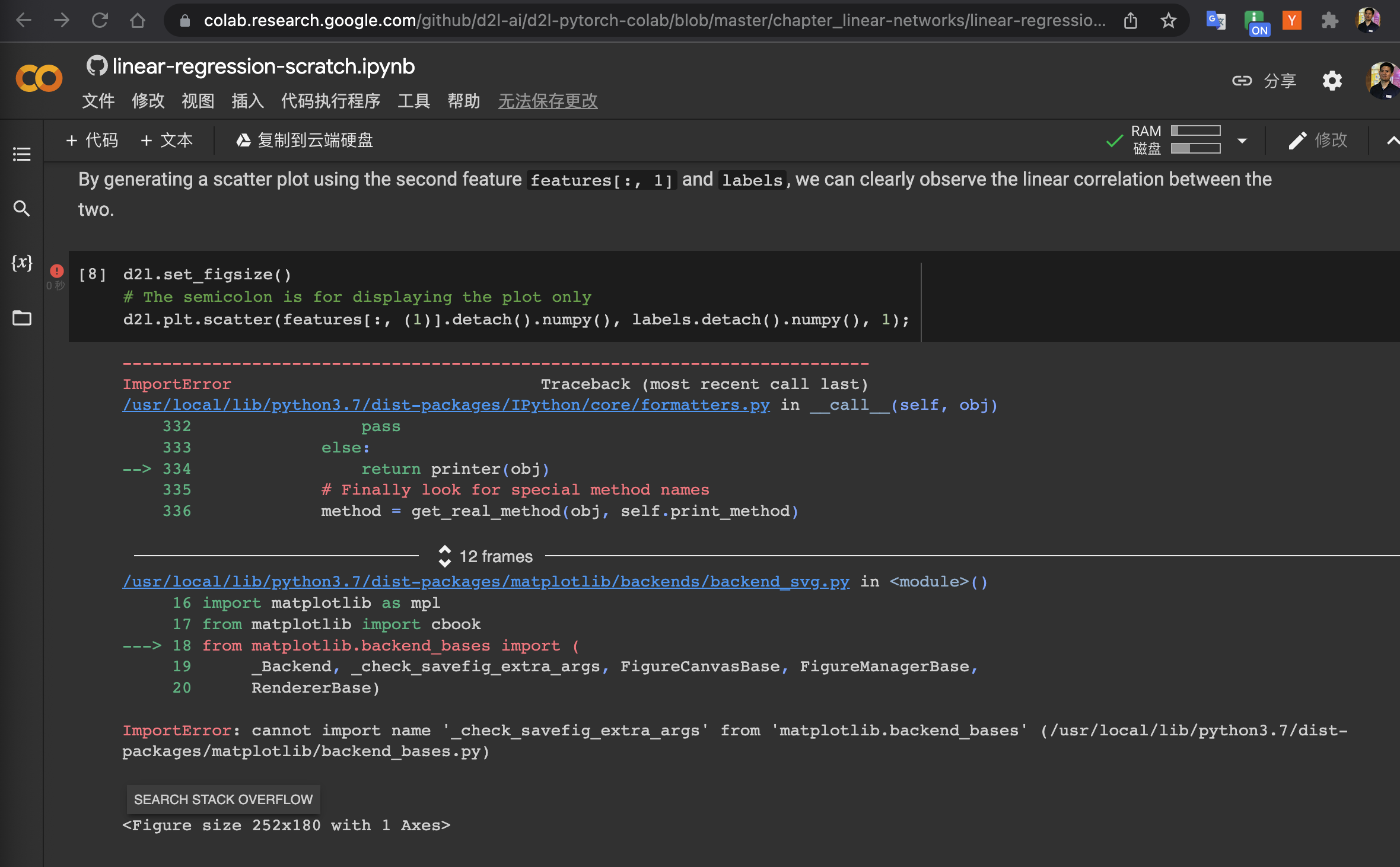
ex.7
I added the code below into the function fit_epoch(), and can see some 8 in the output.

if batch[0].shape[0] != 32:
    print(batch[0].shape[0])

So maybe the data_iter just give out all the examples out to train or validate when the number can’t match the batch size.

ex.8
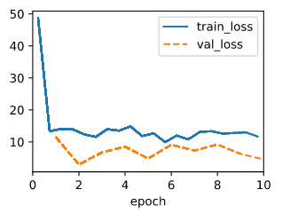
A I tested with those two code snippets below, while the data keeps the same, seems like the training drops sharply at the beginning but then floating near a error that is not that ideal, but the validate eroor is always small than the train error.

@d2l.add_to_class(LinearRegressionScratch)  #@save
def loss(self, y_hat, y):
    l = (y_hat - d2l.reshape(y, y_hat.shape)).abs().sum()
    return l.mean()
model = LinearRegressionScratch(2, lr=0.03, sigma = 0.01)
data = d2l.SyntheticRegressionData(w=torch.tensor([2, -3.4]), b=4.2)
trainer = d2l.Trainer(max_epochs=10)
trainer.fit(model, data)

3

B I use this code to perturb,

data.y[4] = 10000

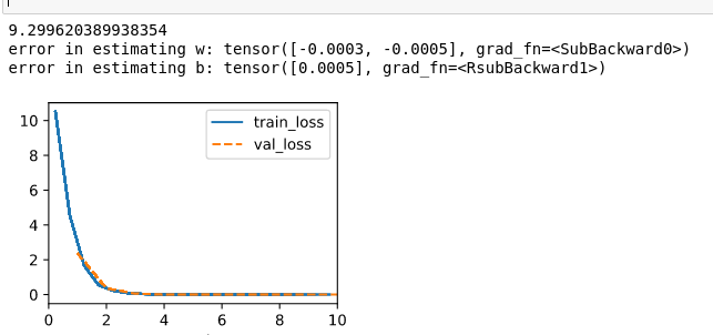
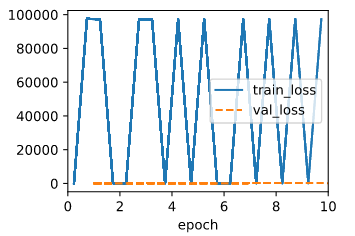
The output for squared loss is:
5
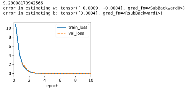
The output for abs loss is:
4
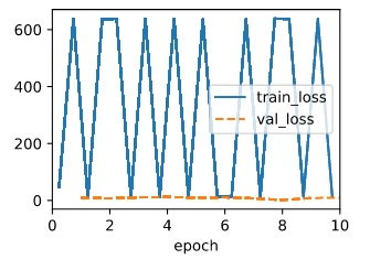
Judging from the result, seems like the squared loss is more vulnerable to large value.

C The abs loss is fast and robust to large value, the squared loss is more accurate.
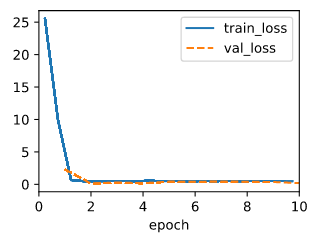
Maybe I can use the sqrt of the mean squared error.

@d2l.add_to_class(LinearRegressionScratch)  #@save
def loss(self, y_hat, y):
    l = (y_hat - y.reshape(y_hat.shape)) ** 2
    l = l.sum().mean().pow(0.5)
    return l

And the test:
6

model = LinearRegressionScratch(2, lr=0.03, sigma = 0.01)
trainer = d2l.Trainer(max_epochs=10)
data = d2l.SyntheticRegressionData(w=torch.tensor([2, -3.4]), b=4.2)
trainer.fit(model, data)

ex.9
I think it’s to break the relation between the data because we don’t need that information.
The shuffle fuction in random package is still run under a predictable formula, so the shuffle is also not that reliable(? I’m not so sure about that).

Like the code I used in ex.2 to produce voltage and current, if I don’t use shuffle, the data will be arranged in the order of the resistor, in other words, the voltage and current get from the same resistor is near to each other.

1 Like

Also confused here, any one has an idea?

IMO the reason is to not track gradients when updating the weights;
With torch.no_grad() block means doing these lines without keeping track of the gradients, in order to not update the gradients when it is updating the weights as that would affect the backdrop.

check this thread

My solutions to the exs: 3.4

because gradient will be accumulated in grad attribute every batch or mini batch by default. see link

Because tensor type is not immutable, python pass it by reference and can change its value inside function. But int type is immutable, python pass it by value and create a new object(int 2) which is then pointed by z in testy2. the value of z outside testy2 is not influenced.

ex.4 your answer is wrong. You can not just backward twice to get 2-order differential. pytorch will accumulate the grad if you do not use grad.zero_()to zero it. Don’t you find the result of the second backward is just twice that of firse backward? You can reference to the code below

 import torch

x = torch.randn((2), requires_grad=True)
y = x**3

dy = torch.autograd.grad(y, x, grad_outputs=torch.ones(x.shape),
                         retain_graph=True, create_graph=True)
dy2 = torch.autograd.grad(dy, x, grad_outputs=torch.ones(x.shape))
2 Likes

Here the code uses a method called “clip_gradients” which involves knowledge about gradient clipping. I searched through the book; this concept is not introduced until 9.5.3. Because this section is to implement linear regression “from scratch”. I suggest we replace this method with something more intuitive for students to understand.

1 Like

Regarding question #7 in the exercises: 7. If the number of examples cannot be divided by the batch size, what happens to data_iter at the end of an epoch?

This topic can be a good teachable moment, but the question needs to be designed more methodically. What happens to a variable in the code is irrelevant here. The real question worth thinking about is - “What should we (or the code) do when a dataset of size M cannot be evenly divided into batches of size N”?

Just thinking about it logically, we have a few options:

A) throw an error
B) force the batch size to closest fit where it evenly divides the dataset
C) divide the dataset and leave one final batch of differing size
D) divide the dataset and trim the final batch of differing size

A) can work, but is not ideal as this problem can be feasibly solved. B) can also work - however in the case where the length of the dataset is a prime number, this effectively will turn mini-batch gradient descent off and just do one big batch with all of the data. For example, a dataset of 101 samples will just be one big batch of 101. This may not be ideal for whoever is using our code.

Ultimately, C) and D) are what it seems modern libraries go for. Pytorch, for example, addresses this in their DataLoader class constructor, specifically the drop_last argument.

Would like for the authors/editors here to be a bit more focused on asking thought-provoking questions and exploring problems (that are pertinent) more deeply. There are a lot of exercises that go way off tangent from the lesson, and others that dive into more advanced topics - which is a problem when you have not ensured that the student has, on a consistent basis, been given the necessary content to master the fundamentals.

2 Likes

In 3.4.2 they say

In the implementation, we need to transform the true value y into the predicted value’s shape y_hat

Isn’t this inconsistent? We should be transforming the predicted value’s shape to the true value right?

with torch.no_grad():
loss.backward()
shouldnt loss.backward be before torch.no_grad

For question 3 in the exercises.
I thought about using a wide range of lambdas and temperatures to calculate the spectral density function then using the temperature as my X or predictor and spectral density function as my y or target.
Am I missing something?

I put this answer for the very first question in the exercise, in case that there are people like me, who (after reading all the discussions about breaking symmetry in weight initialization, etc.) still don’t really understand why initializing weights to zeros still work in this specific exercise, and why it doesn’t work in general.

So, for this specific exercise, where we only try to fit one linear function, it works even if we initialize weight vector with all zeros. Our optimization objective is to minimize weight vector, and the gradient is computed w.r.t weight (dy / dw), which is equal to input vector. Since the gradient is non-zero (and each component in the input vector is probably different from each other), weight is still updated and everything works.

However, for a multi-layer neural network, it doesn’t work anymore, because with a zero weight vector, every hidden layers from the first one will have zero activation values in the first batch, and then continue to have the same value for next batches. Therefore, the gradient flows backward for functions between every hidden layers, as well as output layer will be all the same, leading to the so-called symmetry problem, and that we’re learning the same function for every hidden neurons.

I feel that this Quora answer explains quite well what happens for stubborn head like mine :wink:

1 Like