In section 2.2.3. Conversion to the Tensor Format, the code uses the .values() method, but I believe (at least according to the pandas documentation) that .to_numpy method is now preferred.
The author should consider updating the code to use the pathlib API
import pathlib

dir_out = pathlib.Path().cwd()/'data'
dir_out.mkdir(parents=True, exist_ok=True)
file_new = dir_out / 'tiny.csv'

list_rows = [
    'NumRooms,Alley,Price',  # Column names / Header
    'NA,Pave,127500',  # Each row represents a data example
    '2,NA,106000',
    '4,NA,178100',
    'NA,NA,140000',
    ]

with file_new.open(mode="w") as file:
    for row in list_rows:
        file.write(row + '\n')
If the author wants to suggest pandas, then they should invoke more of the pandas API
inputs = data[['NumRooms', 'Alley']] # dataframe
outputs = data['Price'] # series
Also, calling mean on a whole dataframe will call a future warning unless you specify the operation is on numeric data
inputs.mean(numeric_only=True)
It doesn’t affect these examples, but readers should be aware of this.
You can call them directly as a series then numpy array.
# convert column to tensor
array = data[column_name]
tensor = torch.tensor(array)
By assuming we only want to drop input columns:
data = pd.read_csv(data_file)
inputs, outputs = data.iloc[:, 0:2], data.iloc[:, 2]
nas = inputs.isna().astype(int)
column_index = nas.sum(axis = 0).argmax()
inputs = inputs.drop(inputs.columns[column_index], axis=1)
inputs
Two line code
missingMostColumnIndex = data.count().argmin()
data.drop(columns=data.columns[missingMostColumnIndex])
1. Try loading datasets, e.g., Abalone from the UCI Machine Learning Repository and inspect their properties. What fraction of them has missing values? What fraction of the variables is numerical, categorical, or text?
abalone_data = pd.read_csv("../data/chap_2/abalone.data",
                           names = [
                               "sex", "length", "diameter", "height",
                               "whole_weight", "shucked_weight",
                               "viscera_weight", "shell_weight",
                               "rings"
                           ]
                          )

abalone_data.describe(include = "all")
| sex | length | diameter | height | whole_weight | shucked_weight | viscera_weight | shell_weight | rings | |
|---|---|---|---|---|---|---|---|---|---|
| count | 4177 | 4177.000000 | 4177.000000 | 4177.000000 | 4177.000000 | 4177.000000 | 4177.000000 | 4177.000000 | 4177.000000 |
| unique | 3 | NaN | NaN | NaN | NaN | NaN | NaN | NaN | NaN |
| top | M | NaN | NaN | NaN | NaN | NaN | NaN | NaN | NaN |
| freq | 1528 | NaN | NaN | NaN | NaN | NaN | NaN | NaN | NaN |
| mean | NaN | 0.523992 | 0.407881 | 0.139516 | 0.828742 | 0.359367 | 0.180594 | 0.238831 | 9.933684 |
| std | NaN | 0.120093 | 0.099240 | 0.041827 | 0.490389 | 0.221963 | 0.109614 | 0.139203 | 3.224169 |
| min | NaN | 0.075000 | 0.055000 | 0.000000 | 0.002000 | 0.001000 | 0.000500 | 0.001500 | 1.000000 |
| 25% | NaN | 0.450000 | 0.350000 | 0.115000 | 0.441500 | 0.186000 | 0.093500 | 0.130000 | 8.000000 |
| 50% | NaN | 0.545000 | 0.425000 | 0.140000 | 0.799500 | 0.336000 | 0.171000 | 0.234000 | 9.000000 |
| 75% | NaN | 0.615000 | 0.480000 | 0.165000 | 1.153000 | 0.502000 | 0.253000 | 0.329000 | 11.000000 |
| max | NaN | 0.815000 | 0.650000 | 1.130000 | 2.825500 | 1.488000 | 0.760000 | 1.005000 | 29.000000 |
- There are no items with missing values
- 8 out of 9 attributes are numerical, last is object
2. Try out indexing and selecting data columns by name rather than by column number. The pandas documentation on indexing has further details on how to do this.
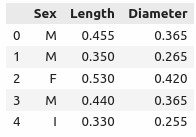
abalone_data[["sex", "rings", "length"]][ : 20]
| sex | rings | length | |
|---|---|---|---|
| 0 | M | 15 | 0.455 |
| 1 | M | 7 | 0.350 |
| 2 | F | 9 | 0.530 |
| 3 | M | 10 | 0.440 |
| 4 | I | 7 | 0.330 |
| 5 | I | 8 | 0.425 |
| 6 | F | 20 | 0.530 |
| 7 | F | 16 | 0.545 |
| 8 | M | 9 | 0.475 |
| 9 | F | 19 | 0.550 |
| 10 | F | 14 | 0.525 |
| 11 | M | 10 | 0.430 |
| 12 | M | 11 | 0.490 |
| 13 | F | 10 | 0.535 |
| 14 | F | 10 | 0.470 |
| 15 | M | 12 | 0.500 |
| 16 | I | 7 | 0.355 |
| 17 | F | 10 | 0.440 |
| 18 | M | 7 | 0.365 |
| 19 | M | 9 | 0.450 |
3.How large a dataset do you think you could load this way? What might be the limitations? Hint: consider the time to read the data, representation, processing, and memory footprint. Try this out on your laptop. What changes if you try it out on a server?
-
How large?
- Depends on the amount of RAM your system has, mine starts struggling at around 8,00,000 records of text data
-
What changes on server?
- If you were using HDD on your machine and SSD on your cloud machine instance/server, you might notice better load times
- Or you might see significantly worse performance since you’re usign free version which has barely more RAM than your machine and uses an HDD to boot

4. How would you deal with data that has a very large number of categories? What if the category labels are all unique? Should you include the latter?
-
If too many categories, try to manually find catgories that are common to each other and group them as one. If they’re all far too different from each other, you’re most likely out of luck, or you can take the information hit and still do the merging of categories to the extent possible
-
If the categories are all unique, meaning number of categories == number of samples in dataset, just drop the column, since the column is carrying no useful information, just like a column that only has 1 value. All values are different(if all unique) or same(if all same) no matter the value of the rest of the attributes, there is no pattern to be found here
5. What alternatives to pandas can you think of? How about loading NumPy tensors from a file? Check out Pillow, the Python Imaging Library.
Just one word : dask ![]()
2 Likes
Create a raw dataset with more rows and columns:
a= [str(x)+’,NA’ for x in list(np.random.randint(0,4, 1000))]
b =[str(y) for y in list(np.random.randint(0,178000, 1000))]
z=[x+’,’+y+’\n’ for (x,y) in zip(a, b)]
with open(data_file, ‘w’) as f:
f.write(‘NumRooms,Alley,Price\n’) # Column names
for x in z:
f.write(x)
-
Delete the column with the most missing values.
d_ict= dict(data.isnull().sum())
max_value = max(d_ict, key=d_ict.get)
data.drop(max_value, axis=1) -
Convert the preprocessed dataset to the tensor format.
outputs, inputs = data.iloc[:,1], data.loc[:,[‘NumRooms’, ‘Price’]]
X, y = torch.tensor(inputs.values), torch.tensor(outputs.values)
X, y
column_names = [“sex”, “length”, “diameter”, “height”, “whole weight”, “shucked weight”, “viscera weight”, “shell weight”, “rings”]
df = pd.read_csv(‘abalone.data’,names=column_names)
print(“Number of samples: %d” % len(df))
df.isna().sum() #Missing values
Catgorical and numerical types
df_numerical = df.select_dtypes(exclude=‘object’)
df_categorical = df.select_dtypes(include=‘object’)
df_numerical_cols = df_numerical.columns.tolist()
df_categorical_cols = df_categorical.columns.tolist()
Indexing can be done:
df.iloc[:,2:][:20]
Ex1.
!wget https://archive.ics.uci.edu/static/public/1/abalone.zip
!unzip abalone.zip
import pandas as pd
attr_names = (
    "Sex", "Length(mm)", "Diameter(mm)", "Height(mm)", "Whole_weight(g)", "Shucked_weight(g)", "Viscera_weight(g)", "Shell_weight(g)", "Rings"
)
# Below shows the most commonly used parameters and kwargs of `pd.read_csv()`
data = pd.read_csv("abalone.data", sep=",", header=None, names=attr_names)
data
Output:
Sex	Length(mm)	Diameter(mm)	Height(mm)	Whole_weight(g)	Shucked_weight(g)	Viscera_weight(g)	Shell_weight(g)	Rings
0	M	0.455	0.365	0.095	0.5140	0.2245	0.1010	0.1500	15
1	M	0.350	0.265	0.090	0.2255	0.0995	0.0485	0.0700	7
2	F	0.530	0.420	0.135	0.6770	0.2565	0.1415	0.2100	9
3	M	0.440	0.365	0.125	0.5160	0.2155	0.1140	0.1550	10
4	I	0.330	0.255	0.080	0.2050	0.0895	0.0395	0.0550	7
...	...	...	...	...	...	...	...	...	...
4172	F	0.565	0.450	0.165	0.8870	0.3700	0.2390	0.2490	11
4173	M	0.590	0.440	0.135	0.9660	0.4390	0.2145	0.2605	10
4174	M	0.600	0.475	0.205	1.1760	0.5255	0.2875	0.3080	9
4175	F	0.625	0.485	0.150	1.0945	0.5310	0.2610	0.2960	10
4176	M	0.710	0.555	0.195	1.9485	0.9455	0.3765	0.4950	12
4177 rows × 9 columns
# Checking missing values in each column, a positive sum indicates the existence of missing entries in a given column
check_na = data.isna()
check_na.sum(axis=0)
Output:
Sex                  0
Length(mm)           0
Diameter(mm)         0
Height(mm)           0
Whole_weight(g)      0
Shucked_weight(g)    0
Viscera_weight(g)    0
Shell_weight(g)      0
Rings                0
dtype: int64
- We don’t have any missing value in this abalone dataset.
- As per the introductory page of the dataset, there are totally 9 attributes (columns), with 8 of them numerical.
- The first column,
Sex, is categorical. We might explore all its possible values via thevalue_counts()method.
categories = data["Sex"].value_counts()
categories
Output:
M    1528
I    1342
F    1307
Name: Sex, dtype: int64
Ex2.
# access a column using dict-like indexing
data["Sex"][0], data.Rings[2]
Output:
('M', 9)
Ex4.
- Too much uniqueness of categorical values indicate that the amount of information that the feature carries is poor. We may safely exclude a feature if all its values are unique.
- Manual or automatic concatenation of categories might be required.
I thank @Tejas-Garhewal for his/her instructive post on this question.
Ex5.
- The
PILlibrary can be used to open an image file as anImageobject; - The
Imageobject can be interpreted as an array, as per the NumPyasarray()method.
Here is the cute cat.png file used. ![]()

from PIL import Image
import numpy as np
img = Image.open("cat.png")
np.asarray(img)
Output:
array([[[199,  56, 130, 255],
        [199,  56, 130, 255],
        [199,  56, 130, 255],
        ...,
        [202,  68, 130, 255],
        [202,  68, 130, 255],
        [202,  68, 130, 255]],

       [[199,  56, 130, 255],
        [199,  56, 130, 255],
        [199,  56, 130, 255],
        ...,
        [202,  68, 130, 255],
        [202,  68, 130, 255],
        [202,  68, 130, 255]],

       [[199,  56, 130, 255],
        [199,  56, 130, 255],
        [199,  56, 130, 255],
        ...,
        [202,  68, 130, 255],
        [202,  68, 130, 255],
        [202,  68, 130, 255]],

       ...,

       [[233, 235, 236, 255],
        [233, 235, 236, 255],
        [233, 235, 236, 255],
        ...,
        [205, 206, 203, 255],
        [204, 206, 203, 255],
        [203, 206, 203, 255]],

       [[233, 235, 236, 255],
        [233, 235, 236, 255],
        [233, 235, 236, 255],
        ...,
        [205, 206, 203, 255],
        [205, 206, 203, 255],
        [204, 206, 203, 255]],

       [[233, 235, 236, 255],
        [233, 235, 236, 255],
        [233, 235, 236, 255],
        ...,
        [205, 206, 203, 255],
        [205, 206, 203, 255],
        [205, 206, 203, 255]]], dtype=uint8)
”“”Depending upon the context, missing values might be handled either via imputation or deletion . Imputation replaces missing values with estimates of their values while deletion simply discards either those rows or those columns that contain missing values.“”“
I think “imputation” should be changed to “Interpolation”.
I think the correct code for the pd.get_dummies function is the following:
inputs = pd.get_dummies(inputs,columns=['RoofType'],dummy_na=True)
Hi!
Link to Abalone dataset is broken. Here’s the correct one:
2 Likes
I went through these exercises a week or so ago and can’t find the notes I took. From what I recall:
- The dataset I downloaded had a decently high fraction of missing values (~10%?). The dataset was predominantly numerical and categorical (maybe 50/50). No text fields.
- You can do this by bracketed indexing (e.g.
data['column_name']or with the.locaccessor (e.g.data.loc[:, 'column_name']). - I ran some experiments on my laptop by writing a Go program to generate a large (~30 GB) csv dataset. Reading the csv into memory was quite slow – something like 30 MB/second, despite a relatively fast SSD on my computer. This may have had to do with the content, and I imagine this would be much slower on an HDD. The ultimate bottleneck was RAM. It seems that Pandas loads the entire dataset into RAM, which meant I had to stop after ~16 GB.
- I don’t really understand this question. You can include them, or not. Depends on what you’re using the data for.
- I’ve heard great things about Polars. In practice, I tend to use sqlite3 for most light-medium data workloads.
Exercise 1
import pandas as pd

URL = "https://archive.ics.uci.edu/ml/machine-learning-databases/abalone/abalone.data"
cols = ["Sex", "Length", "Diameter", "Height", "Whole_weight",
        "Shucked_weight", "Viscera_weight", "Shell_weight", "Rings"]
abalone = pd.read_csv(URL, names=cols)
abalone.isna().mean()
Sex               0.0
Length            0.0
Diameter          0.0
Height            0.0
Whole_weight      0.0
Shucked_weight    0.0
Viscera_weight    0.0
Shell_weight      0.0
Rings             0.0
dtype: float64
num = round(abalone.select_dtypes(include=["number"]).shape[1] / abalone.shape[1], 3)
cat = round(abalone.select_dtypes(include=["object"]).shape[1] / abalone.shape[1], 3)
num, cat
(0.889, 0.111)
Exercise 2
abalone[["Sex", "Length", "Diameter"]].head() # == abalone.iloc[:, :3].head()
Exercise 3
import numpy as np
import psutil
import time

def memory_usage():
    memory = psutil.virtual_memory()
    print(f"Total system memory: {memory.total / (1024 ** 3):.2f} GB")
    print(f"Used memory: {memory.used / (1024 ** 3):.2f} GB")
    print(f"Available memory: {memory.available / (1024 ** 3):.2f} GB")

sizes = [10, 100, 1000]
for size in sizes:
    print(f"> Loading {size} million rows of data.")
    start_time = time.time()
    df = pd.DataFrame({"random": np.random.randn(size * 10 ** 6)})
    memory_usage()
    elapsed_time = time.time() - start_time
    print(f"Elapsed time: {elapsed_time:.2f} seconds\n")
    del df
> Loading 10 million rows of data.
Total system memory: 19.23 GB
Used memory: 2.58 GB
Available memory: 15.72 GB
Elapsed time: 0.15 seconds

> Loading 100 million rows of data.
Total system memory: 19.23 GB
Used memory: 3.26 GB
Available memory: 15.04 GB
Elapsed time: 1.42 seconds

> Loading 1000 million rows of data.
Total system memory: 19.23 GB
Used memory: 9.82 GB
Available memory: 8.48 GB
Elapsed time: 16.46 seconds
- The time to load the data increases with the size of the dataset. For example, loading 10 million rows took 0.15 seconds, while 1 billion rows took 16.46 seconds.
- The larger the dataset, the more memory is used. This can lead to excessive consumption of the available memory.
- Large datasets require more CPU and memory resources, which can overload the system, especially on PCs with fewer resources (as in my case).
- On my laptop, the ability to load data is limited by memory and processing power. Loading 1 billion rows used almost half of the available memory.Servers have more resources and can handle larger datasets more efficiently, but they still have memory and processing limits.
Exercise 4
- For data with a very large number of categories, we could use frequency encoding or mean encoding.
- If the category labels are all unique, we could consider grouping by similar categories (for example, if it’s a city area code, we would group by region), or discard it if this feature does not provide any generalizable information.
Exercise 5
- There are several alternatives to Pandas, such as Polars, which claim to process large DataFrames faster. Other options can be found in the list on Kyle Mitchell’s repository.
np.random.seed(42)
PATH_FILE = "../data/example.npy"
np.save(PATH_FILE, np.random.rand(100, 100))
np.load(PATH_FILE)
array([[0.37454012, 0.95071431, 0.73199394, ..., 0.42754102, 0.02541913,
        0.10789143],
       [0.03142919, 0.63641041, 0.31435598, ..., 0.89711026, 0.88708642,
        0.77987555],
       [0.64203165, 0.08413996, 0.16162871, ..., 0.21582103, 0.62289048,
        0.08534746],
       ...,
       [0.78073273, 0.21500477, 0.71563555, ..., 0.64534562, 0.4147358 ,
        0.93035118],
       [0.78488298, 0.20000892, 0.13084236, ..., 0.67981813, 0.83092249,
        0.04159596],
       [0.02311067, 0.3730071 , 0.14878828, ..., 0.94670792, 0.39748799,
        0.2171404 ]])
1 Like
Ex. 1. Here’s the program to load the Abalone dataset, with the dataset taken from the abalon.data file and column names - from the abalon.names file:
import pandas as pd
column_names = [
    'Sex',
    'Length',
    'Diameter',
    'Height',
    'Whole weight',
    'Shucked weight',
    'Viscera weight',
    'Shell weight',
    'Rings'
]
data_file = 'abalone.data'
data = pd.read_csv(data_file, names = column_names)
# print(data)
missing_values_absolute = data.isnull().sum()

# Calculate the ratio of missing values for each column
missing_values_ratio = (data.isnull().sum() / len(data)) * 100

missing_data = pd.DataFrame({
    'Missing Values': missing_values_absolute,
    'Percentage (%)': missing_values_ratio
})

print(missing_data)
                Missing Values  Percentage (%)
Sex                          0             0.0
Length                       0             0.0
Diameter                     0             0.0
Height                       0             0.0
Whole weight                 0             0.0
Shucked weight               0             0.0
Viscera weight               0             0.0
Shell weight                 0             0.0
Rings                        0             0.0
What fraction of them has missing values?
0% of the values are missing.
What fraction of the variables is numerical, categorical, or text?
Here’s the description of the columns from the abalone.names file:
	----		---------	-----	-----------
	Sex		nominal			M, F, and I (infant)
	Length		continuous	mm	Longest shell measurement
	Diameter	continuous	mm	perpendicular to length
	Height		continuous	mm	with meat in shell
	Whole weight	continuous	grams	whole abalone
	Shucked weight	continuous	grams	weight of meat
	Viscera weight	continuous	grams	gut weight (after bleeding)
	Shell weight	continuous	grams	after being dried
	Rings		integer			+1.5 gives the age in years```

Result:
0.1 of the properties are categorical
0.8 of the properties are float numbers
0.1 of the properties are integer numbers

Ex. 2. **Try indexing and selecting data columns by name rather than by column number.**
Here's the code example for this:
import pandas as pd
column_names = [
‘Sex’,
‘Length’,
‘Diameter’,
‘Height’,
‘Whole weight’,
‘Shucked weight’,
‘Viscera weight’,
‘Shell weight’,
‘Rings’
]
data_file = ‘abalone.data’
data = pd.read_csv(data_file, names = column_names)
inputs, targets = data.loc[:, ‘Sex’:‘Shell weight’], data.loc[:, ‘Rings’]
print(f’Inputs={inputs}‘)
print(f’Targets={targets}’)
Here's the output:
Inputs= Sex Length Diameter … Shucked weight Viscera weight Shell weight
0 M 0.455 0.365 … 0.2245 0.1010 0.1500
1 M 0.350 0.265 … 0.0995 0.0485 0.0700
2 F 0.530 0.420 … 0.2565 0.1415 0.2100
3 M 0.440 0.365 … 0.2155 0.1140 0.1550
4 I 0.330 0.255 … 0.0895 0.0395 0.0550
… … … … … … … …
4172 F 0.565 0.450 … 0.3700 0.2390 0.2490
4173 M 0.590 0.440 … 0.4390 0.2145 0.2605
4174 M 0.600 0.475 … 0.5255 0.2875 0.3080
4175 F 0.625 0.485 … 0.5310 0.2610 0.2960
4176 M 0.710 0.555 … 0.9455 0.3765 0.4950
[4177 rows x 8 columns]
Targets=0 15
1 7
2 9
3 10
4 7
…
4172 11
4173 10
4174 9
4175 10
4176 12
Ex. 2. Try indexing and selecting data columns by name rather than by column number.
Here’s the code example for this:
import pandas as pd
column_names = [
    'Sex',
    'Length',
    'Diameter',
    'Height',
    'Whole weight',
    'Shucked weight',
    'Viscera weight',
    'Shell weight',
    'Rings'
]
data_file = 'abalone.data'
data = pd.read_csv(data_file, names = column_names)


inputs, targets = data.loc[:, 'Sex':'Shell weight'], data.loc[:, 'Rings']


print(f'Inputs={inputs}')
print(f'Targets={targets}')
Here’s the output:
Inputs=     Sex  Length  Diameter  ...  Shucked weight  Viscera weight  Shell weight
0      M   0.455     0.365  ...          0.2245          0.1010        0.1500
1      M   0.350     0.265  ...          0.0995          0.0485        0.0700
2      F   0.530     0.420  ...          0.2565          0.1415        0.2100
3      M   0.440     0.365  ...          0.2155          0.1140        0.1550
4      I   0.330     0.255  ...          0.0895          0.0395        0.0550
...   ..     ...       ...  ...             ...             ...           ...
4172   F   0.565     0.450  ...          0.3700          0.2390        0.2490
4173   M   0.590     0.440  ...          0.4390          0.2145        0.2605
4174   M   0.600     0.475  ...          0.5255          0.2875        0.3080
4175   F   0.625     0.485  ...          0.5310          0.2610        0.2960
4176   M   0.710     0.555  ...          0.9455          0.3765        0.4950

[4177 rows x 8 columns]
Targets=0       15
1        7
2        9
3       10
4        7
        ..
4172    11
4173    10
4174     9
4175    10
4176    12
Ex. 3. 1. How large a dataset do you think you could load this way? What might be the limitations? Hint: consider the time to read the data, representation, processing, and memory footprint. Try this out on your laptop. What happens if you try it out on a server?
The limitations might be: CPU capacity, RAM capacity, and data loading time.
Here’s the program to check memory utilization, for example. It loads a random dataset with a progressively growing number of rows and a constant number of columns.
import pandas as pd
import numpy as np
import time
import os
import psutil

# Function to get current memory usage in MB
def get_memory_usage():
    process = psutil.Process(os.getpid())
    return process.memory_info().rss / 1024**2  # Convert to MB

# Function to get total system memory in MB
def get_total_memory():
    return psutil.virtual_memory().total / 1024**2  # Convert to MB

# Function to estimate the memory required for the DataFrame
def estimate_memory_usage(rows, cols, dtype=np.float64):
    # Memory in bytes: number of elements * size of each element
    return rows * cols * np.dtype(dtype).itemsize / 1024**2  # Convert to MB

# Main function
def progressively_load_data(max_n=7, memory_threshold=80):
    total_memory = get_total_memory()
    print(f"Total system memory: {total_memory:.2f} MB\n")

    for N in range(1, max_n + 1):
        rows = 10**N
        cols = 10

        # Estimate the memory required to create the DataFrame
        required_memory = estimate_memory_usage(rows, cols)

        if required_memory > (total_memory * (memory_threshold / 100)):
            print(f"Iteration {N}: Estimated memory usage of {required_memory:.2f} MB exceeds the threshold. Stopping to prevent freezing.")
            break

        print(f"Iteration {N}: Loading DataFrame with {rows} rows and {cols} columns")
        print(f"Estimated memory usage: {required_memory:.2f} MB")

        start_time = time.time()

        # Generate DataFrame with random numbers
        large_data = pd.DataFrame(np.random.rand(rows, cols), columns=[f'col_{i}' for i in range(cols)])

        end_time = time.time()
        elapsed_time = end_time - start_time
        memory_usage = get_memory_usage()

        print(f"Time elapsed: {elapsed_time:.2f} seconds")
        print(f"Memory usage: {memory_usage:.2f} MB")

        print("-" * 50)

if __name__ == "__main__":
    progressively_load_data(max_n=16, memory_threshold=80)
Output:
Total system memory: 15707.79 MB

Iteration 1: Loading DataFrame with 10 rows and 10 columns
Estimated memory usage: 0.00 MB
Time elapsed: 0.00 seconds
Memory usage: 59.25 MB
--------------------------------------------------
Iteration 2: Loading DataFrame with 100 rows and 10 columns
Estimated memory usage: 0.01 MB
Time elapsed: 0.00 seconds
Memory usage: 59.25 MB
--------------------------------------------------
Iteration 3: Loading DataFrame with 1000 rows and 10 columns
Estimated memory usage: 0.08 MB
Time elapsed: 0.00 seconds
Memory usage: 59.25 MB
--------------------------------------------------
Iteration 4: Loading DataFrame with 10000 rows and 10 columns
Estimated memory usage: 0.76 MB
Time elapsed: 0.00 seconds
Memory usage: 60.03 MB
--------------------------------------------------
Iteration 5: Loading DataFrame with 100000 rows and 10 columns
Estimated memory usage: 7.63 MB
Time elapsed: 0.00 seconds
Memory usage: 67.02 MB
--------------------------------------------------
Iteration 6: Loading DataFrame with 1000000 rows and 10 columns
Estimated memory usage: 76.29 MB
Time elapsed: 0.04 seconds
Memory usage: 135.69 MB
--------------------------------------------------
Iteration 7: Loading DataFrame with 10000000 rows and 10 columns
Estimated memory usage: 762.94 MB
Time elapsed: 0.39 seconds
Memory usage: 822.46 MB
--------------------------------------------------
Iteration 8: Loading DataFrame with 100000000 rows and 10 columns
Estimated memory usage: 7629.39 MB
Time elapsed: 5.83 seconds
Memory usage: 7439.57 MB
--------------------------------------------------
Iteration 9: Estimated memory usage of 76293.95 MB exceeds the threshold. Stopping to prevent freezing.
Conclusion: RAM is more sensitive to dataframe size than execution time.
It’s possible to load more data within the same RAM by changing data type. The default is float64 but we can change to float32 by changing this line:
required_memory = estimate_memory_usage(rows, cols)
to
required_memory = estimate_memory_usage(rows, cols, dtype=np.float32)
and
large_data = pd.DataFrame(np.random.rand(rows, cols), columns=[f'col_{i}' for i in range(cols)])
to
large_data = pd.DataFrame(np.random.rand(rows, cols).astype(np.float32), columns=[f'col_{i}' for i in range(cols)])
This approach allows loading as much as 100000000 rows.
Output:
Iteration 7: Loading DataFrame with 10000000 rows and 10 columns
Estimated memory usage: 381.47 MB
Time elapsed: 0.48 seconds
Memory usage: 441.57 MB
--------------------------------------------------
Iteration 8: Loading DataFrame with 100000000 rows and 10 columns
Estimated memory usage: 3814.70 MB
Time elapsed: 21.80 seconds
Memory usage: 2950.52 MB
--------------------------------------------------
Iteration 9: Estimated memory usage of 38146.97 MB exceeds the threshold. Stopping to prevent freezing.
use candle and polars to show DataPreprocessing
use std::io::Write;

use polars::prelude::*;

use candle_core::{Device, Tensor};

fn main() -> Result<(), Box<dyn std::error::Error>> {
    let data_dir = std::path::Path::new("..").join("data");
    if !std::fs::exists(data_dir.clone())? {
        std::fs::create_dir(data_dir.clone())?;
    }

    let data_file = data_dir.join("house_tiny.csv");
    let mut buffer = std::fs::File::create(data_file.clone())?;
    write!(
        buffer,
        r#"NumRooms,RoofType,Price
NA,NA,127500
2,NA,106000
4,Slate,178100
NA,NA,140000"#
    )?;
    buffer.sync_all()?;

    let df1 = polars::prelude::CsvReadOptions::default()
        .with_has_header(true)
        .try_into_reader_with_file_path(data_file.into())?
        .finish()?;

    println!("{}", df1);

    let df2 = df1
        .clone()
        .lazy()
        .select([
            when(col("NumRooms").eq(lit("NA")))
                .then(lit(NULL))
                .otherwise(col("NumRooms"))
                .cast(DataType::Float32)
                .alias("NumRooms"),
            when(col("RoofType").eq(lit("NA")))
                .then(lit(NULL))
                .otherwise(col("RoofType"))
                .alias("RoofType"),
            col("Price").cast(DataType::Float32),
        ])
        .collect()?;
    println!("{}", df2);

    let inputs = df2
        .clone()
        .lazy()
        .select([
            col("NumRooms")
                .fill_null(col("NumRooms").mean())
                .alias("NumRooms"),
            when(col("RoofType").is_null())
                .then(0_)
                .otherwise(1)
                .cast(DataType::Float32)
                .alias("RoofType_Slate"),
            when(col("RoofType").is_null())
                .then(1)
                .otherwise(0)
                .cast(DataType::Float32)
                .alias("RoofType_Nan"),
        ])
        .collect()?;
    println!("inputs:\n{}", inputs);

    let target = df2.clone().lazy().select([col("Price")]).collect()?;
    println!("target:\n{}", target);

    let cpu = Device::Cpu;
    let input_buffer = inputs.to_ndarray::<Float32Type>(IndexOrder::C)?;
    let x_tensor = Tensor::from_slice(input_buffer.as_slice().unwrap(), inputs.shape(), &cpu)?;
    let y_tensor = Tensor::from_slice(
        target
            .to_ndarray::<Float32Type>(IndexOrder::C)?
            .as_slice()
            .unwrap(),
        target.shape(),
        &cpu,
    )?
    .transpose(0, 1)?;

    println!("x tensor:\n{x_tensor}");
    println!("y tensor:\n{y_tensor}");

    Ok(())
}
Q1. Try loading datasets, e.g., Abalone from the UCI Machine Learning Repository 50 and inspect their properties. What fraction of them has missing values? What fraction of the variables is numerical, categorical, or text? (Ex. 2.2.5)
uci = "abalone/abalone.data"
uci_data = pd.read_csv(uci)
uci_data.head(10)
M 0.455 0.365 0.095 0.514 0.2245 0.101 0.15 15 0 M 0.350 0.265 0.090 0.2255 0.0995 0.0485 0.070 7 1 F 0.530 0.420 0.135 0.6770 0.2565 0.1415 0.210 9 2 M 0.440 0.365 0.125 0.5160 0.2155 0.1140 0.155 10 3 I 0.330 0.255 0.080 0.2050 0.0895 0.0395 0.055 7 4 I 0.425 0.300 0.095 0.3515 0.1410 0.0775 0.120 8 5 F 0.530 0.415 0.150 0.7775 0.2370 0.1415 0.330 20 6 F 0.545 0.425 0.125 0.7680 0.2940 0.1495 0.260 16 7 M 0.475 0.370 0.125 0.5095 0.2165 0.1125 0.165 9 8 F 0.550 0.440 0.150 0.8945 0.3145 0.1510 0.320 19 9 F 0.525 0.380 0.140 0.6065 0.1940 0.1475 0.210 14
colnames = pd.read_csv("Book1.csv", header=None)
colnames
0 0 sex 1 length 2 diameter 3 height 4 whole_weight 5 shucked_weight 6 viscera_weight 7 shell_weight 8 rings
labels = colnames.iloc[:, 0]
labels
0 sex
1 length
2 diameter
3 height
4 whole_weight
5 shucked_weight
6 viscera_weight
7 shell_weight
8 rings
Name: 0, dtype: object
new_uci = uci_data.set_axis(labels, axis=1)
new_uci.head(10)
sex length diameter height whole_weight shucked_weight viscera_weight shell_weight rings 0 M 0.350 0.265 0.090 0.2255 0.0995 0.0485 0.070 7 1 F 0.530 0.420 0.135 0.6770 0.2565 0.1415 0.210 9 2 M 0.440 0.365 0.125 0.5160 0.2155 0.1140 0.155 10 3 I 0.330 0.255 0.080 0.2050 0.0895 0.0395 0.055 7 4 I 0.425 0.300 0.095 0.3515 0.1410 0.0775 0.120 8 5 F 0.530 0.415 0.150 0.7775 0.2370 0.1415 0.330 20 6 F 0.545 0.425 0.125 0.7680 0.2940 0.1495 0.260 16 7 M 0.475 0.370 0.125 0.5095 0.2165 0.1125 0.165 9 8 F 0.550 0.440 0.150 0.8945 0.3145 0.1510 0.320 19 9 F 0.525 0.380 0.140 0.6065 0.1940 0.1475 0.210 14
X = pd.get_dummies(X, dummy_na = False)
X.head(10)
length diameter height whole_weight shucked_weight viscera_weight shell_weight sex_F sex_I sex_M 0 0.350 0.265 0.090 0.2255 0.0995 0.0485 0.070 False False True 1 0.530 0.420 0.135 0.6770 0.2565 0.1415 0.210 True False False 2 0.440 0.365 0.125 0.5160 0.2155 0.1140 0.155 False False True 3 0.330 0.255 0.080 0.2050 0.0895 0.0395 0.055 False True False 4 0.425 0.300 0.095 0.3515 0.1410 0.0775 0.120 False True False 5 0.530 0.415 0.150 0.7775 0.2370 0.1415 0.330 True False False 6 0.545 0.425 0.125 0.7680 0.2940 0.1495 0.260 True False False 7 0.475 0.370 0.125 0.5095 0.2165 0.1125 0.165 False False True 8 0.550 0.440 0.150 0.8945 0.3145 0.1510 0.320 True False False 9 0.525 0.380 0.140 0.6065 0.1940 0.1475 0.210 True False False
X.isna().any()
length False
diameter False
height False
whole_weight False
shucked_weight False
viscera_weight False
shell_weight False
sex_F False
sex_I False
sex_M False
dtype: bool
This datset has no NaN values. 1/9 columns is categorical and the rest are all numerical values.