I feel puzzled about Q1. If we replace nn.MSELoss(reduction='sum') with nn.MSELoss() and we want the code to behave identically, I think we need to replace ‘lr’ with ‘lr/batch_size’. However, the result seems different. Can anyone tell me what’s wrong here?
4 Likes
I had the same intuition and ran into the same issues on Q1. The question for the MXNET implementation suggested to me that that approach (dividing by batch size) might be correct, but I’ve had no luck so far finding a learning rate that produces results even close to those obtained using the default reduction (mean).
MXNET question, for reference:
If we replace
l = loss(output, y)withl = loss(output, y).mean(), we need to changetrainer.step(batch_size)totrainer.step(1)for the code to behave identically. Why?
edit to updated with further progress
I wasn’t paying enough attention to the code. Dividing the step size by 10 doesn’t account for the fact that the loss that’s actually printed incorporates all 1000 observations. So I was consistently off by a factor of 1000 by not dividing loss(net(features), labels) by 1000 when using sum and comparing to the loss using mean. After incorporating this change, dividing the learning rate by the batch size had the desired results (or at least the same order of magnitude; I haven’t made a single version of this working on exactly the same data as I’m still pretty uncertain about automatic differentiation).
So my big question now is: am I still missing something big? I was unable to find a way get the same output using mean and sum reduction changing only the learning rate. Is there a way to do so? I experimented with many different values and was unable to find a way.
Another edit with more testing
I ran the comparison after setting a random seed and was able to obtain identical (not just same order of magnitude) results with reduction='sum' by dividing the learning rate by the batch size and by changing the per-epoch loss calculation to l = loss(net(features), labels)/1000.
The results were not identical when I changed the learning rate to any other value. So I’ve mostly convinced myself that this approach is correct, and it makes intuitive sense to me. But I do think the question implied this could be solved by changing only the learning rate, so I still wonder if I’m missing something there.
Hi @dliden, I think the nature of loss function is not changed whatever you set the reduction to ‘sum’ or ‘mean’. And I think the difference between ‘sum’ and ‘mean’ is loss_mean = loss_sum/1000. Such that when the reduction is set to ‘sum’, the loss is sensitive for a little change of weights. In other words, even if you update the weights a little, the loss will change greatly. What’s worse, you could skip the minimum and the training will never converge. Therefore, you should change the learning rate smaller. Try to set the lr=0.001 and num_epochs=10, you will something different.
Did you set a seed to ensure reproducibility? Before generating random numbers, you should set a seed for NumPy and PyTorch, like this:
np.random.seed(868990)
torch.manual_seed(868990)
Choose a number you like – I chose the years Greg LeMond won the Tour de France.
Then you should see the same results. Note: the magnitudes for the loss will be different because of mean vs. sum.
It is already correct, and to get the correct result you should divide the loss value to the length of the features.
1 Like
Hi Goldpiggy,
For question 1
how can we change the learning rate for the code to behave identically. Why?
I’m very confused why the learning rate is affected when we set reduction = sum. I have read through the thread and seems they were not talking about the learning rate. I made some experiments and found the training loss was increased tremendously when we set it as sum. Could you explain that to me. Thanks ![]()
As we have specified the input and output dimensions when constructing
nn.Linear.
Incomplete sentence. As we have done this, so what? Perhaps remove the first word?
Here are my opinions for exs:
If you got any better idea please tell me ,thanks a lot.
Note that I still can’t work out ex.3, and not so sure about ex.5.
ex.1
To get the aggregate loss, I multiply the number of minibatch(X.shape[0]):
@d2l.add_to_class(LinearRegression)  #@save
def forward(self, X):
    """The linear regression model."""
    #return self.net(X)
    return self.net(X)*X.shape[0]
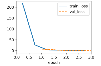
When using the old lr=0.03, the ouput is:
That means the lr is too large, so I divide the lr by the number of minibatch, and the ouput becomes normal.
#model = LinearRegression(lr=0.03)
model = LinearRegression(lr=0.03/1000.)
data = d2l.SyntheticRegressionData(w=torch.tensor([2, -3.4]), b=4.2)
trainer = d2l.Trainer(max_epochs=3)
trainer.fit(model, data)
But after read @hy38’s reply I think It’s better to set the paramter reduction=‘sum’ to do that. ![]()
ex.2
?nn.MSELoss
??nn.modules.loss
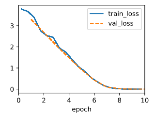
By search the nn.MSELoss, I find it’s definition path is “…/torch/nn/modules/loss.py”, so I scan this path, and search with keyword ‘Huber’ and find ‘class HuberLoss(_Loss)’, then I test with this code, seems like the Huber’s robust loss regress slower(10 epochs rather than 3 epochs) than the MSELoss and the two errors is close.
@d2l.add_to_class(LinearRegression)  #@save
def loss(self, y_hat, y):
    fn = nn.HuberLoss()
    return fn(y_hat, y)

model = LinearRegression(lr=0.03)
data = d2l.SyntheticRegressionData(w=torch.tensor([2, -3.4]), b=4.2)
trainer = d2l.Trainer(max_epochs=10)
trainer.fit(model, data)

print(f'error in estimating w: {data.w - w.reshape(data.w.shape)}')
print(f'error in estimating b: {data.b - b}')
error in estimating w: tensor([ 0.0125, -0.0156])
error in estimating b: tensor([0.0138])
ex.3
After scanning the doc of torch.optim.SGD, I find that the grad is not a self. like parameters, and I can’t find a function to fetch the gard. ![]()
ex.4
I test with this code snippet:
lrs = [3,0.3,0.03,0.003]
for lr in lrs:
    model = LinearRegression(lr)
    data = d2l.SyntheticRegressionData(w=torch.tensor([2, -3.4]), b=4.2)
    trainer = d2l.Trainer(max_epochs=10)
    trainer.fit(model, data)
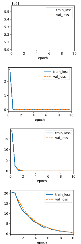
Seems like lr=3 is too large that it may produce a lot NaN when computing loss, 0.003 is too small, 0.3 is better than the original 0.03.
ex.5
A. I use this code snippet:
def ex5_20220905(data_sizes, model, trainer):
    w_errs = list()
    b_errs = list()
    for data_size in data_sizes:
        data_size = int(data_size)
        data = d2l.SyntheticRegressionData(w=torch.tensor([2, -3.4]), b=4.2,
                                           num_train=data_size, num_val=data_size)
        trainer.fit(model, data)
        w, b = model.get_w_b()
        w_errs.append(data.w - w.reshape(data.w.shape))
        b_errs.append(data.b - b)
    return w_errs, b_errs

data_sizes = torch.arange(2,2+5,1)
data_sizes = torch.log(data_sizes)*1000
model = LinearRegression(lr=0.03)
trainer = d2l.Trainer(max_epochs=3)
w_errs, b_errs = ex5_20220905(data_sizes=data_sizes, model= model, trainer=trainer)
print(f'data size\tw error\t\t\tb error')
for i in range(len(data_sizes)):
    print(f'{int(data_sizes[i])}\t{w_errs[i]}\t\t\t{b_errs[i]}')
| data size | w error | b error | ||
|---|---|---|---|---|
| 693 | tensor([ 0.0563, -0.0701]) | tensor([0.0702]) | ||
| 1098 | tensor([ 0.0002, -0.0004]) | tensor([7.6771e-05]) | ||
| 1386 | tensor([-0.0010, 0.0001]) | tensor([-0.0005]) | ||
| 1609 | tensor([ 0.0006, -0.0001]) | tensor([0.0003]) | ||
| 1791 | tensor([ 1.8096e-04, -4.1723e-05]) | tensor([-4.0531e-05]) |
B. Judging from the data above, I think the logarithm growing for data size is more economic way to find a appropriate size of data, because as the data size grows, the same number of data added to the dataset receive less and less effect to reduce the error.(??I’m not so sure about that.)
2 Likes
I have a question about the initialization of the lazy layer parameters. As i know in the pytorch doc, the lazy layer parameters are torch.nn.parameter.UninitializedParameter that can’t have operations on them. why there’s initializations on them?
In the PyTorch code, the initializations in 3.5.1 will not work - when using nn.LazyLinear, the .weight.data will be uninitialized until the first call to forward(), meaning the .normal_ and .fill_ calls are noops. These initializations silently fail! This is why I prefer to avoid LazyLinear - it can lead to subtle bugs.
1 Like
- To maintain the update size while switching from aggregate to mean loss, you’d multiply the learning rate by
n(the number of samples per minibatch). - Huber loss is a drop-in replacement (
torch.nn.HuberLoss()), but leads to slower convergence here. This makes sense when you consider that outside of the range defined by\delta, Huber loss is equivalent to MAE loss, for which the magnitude of the gradients are constant (whereas the MSE loss we were using earlier punishes outliers by a quadratic factor). model.net.weight.grad- Learning rate affects the time to convergence (within reasonable bounds, causing failure to train outside of them). With more epochs, the model makes better approximations of the true values up to a certain point - it’ll converge on the true values relative to the dataset, which may slightly differ from our “original values” because of the Gaussian noise we added.
- As one might expect - ceteris paribus, a model trained on more data will converge in fewer epochs. The suggestion on the hint is appropriate because we’d practically be looking for the right order of magnitude of the data. This will typically yield a more meaningful trend for most statistical estimators, since the variance scales with
1/\sqrt{n}.
ex 2
we can use dir(torch.nn) and search huber loss in the result, and we’ll find HuberLoss
So We can use torch.nn.HuberLoss for this exercise.
ex 3
the params’ info should be found in model.net
To be specific, we can look into nn.Parameter for our answer. In the example, we can use model.net.weight.grad to check the gradient. Need to be noted that we shouldn’t use model.net.weight.data.grad, which is always None since all autograd has been recorded in Parameter.grad instead of Parameter.data.grad
but I have a problem:
In my IDE (Jetbrains IDEA with Python, Jupyter plugin enabled) the interactive plotting for training didn’t work fine: it won’t draw.
In my browser (Chrome), the interactive plotting for training works, but for every iteration draw, it’ll clear the output, which means I can’t see output text after a graph is drawn, and I can’t do multiple experiments in the same cell like @GpuTooExpensive does in his/hers ex 4.
thanks a lot! ![]()