I’m confused with partial derivatives. Since for partial derivatives we can treat all other variables as constants, shouldn’t the derivative vector be [6x_1, 5e^x_2] ?
∂f/∂x_1 = ∂/∂x_1 (3x_1^2) + DC = 6x_1 + 0 = 6x_1 (C being a constant)
1 Like
I believe the F implies the Frobenius Norm:http://d2l.ai/chapter_preliminaries/linear-algebra.html?highlight=norms
I’m not clear on what the notation implies when there is both a subscript F and a superscript 2. The text reads as if the Frobenius Norm is always the square root of the sum of its matrix elements, so the superscript should always be 2. Is this understanding incorrect?
pbouzon
November 8, 2021, 10:11pm
23
Exercise 2:x ) = [6x1, 5e^x2]
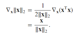
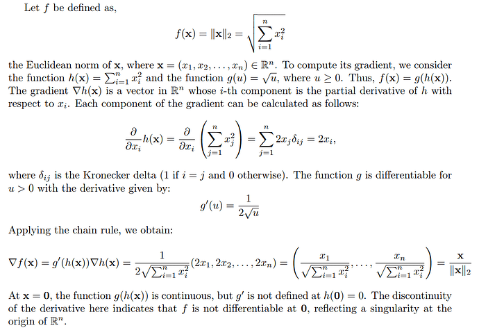
Exercise 3:x ) = (x1² + x2² … + xn²)¹/²x ) = x /f(x )
Exercise 4:
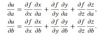
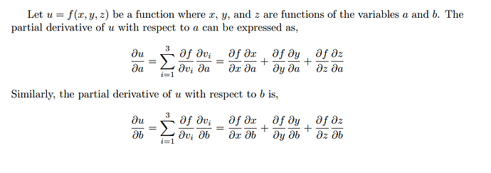
du/da = (du/dx)(dx/da) + (du/dy)(dy/da) + (du/dz)(dz/da)
2 Likes
The superscript 2 means you are squaring the Forbenius Norm. So, the square root in the Forbenius Norm disappears.
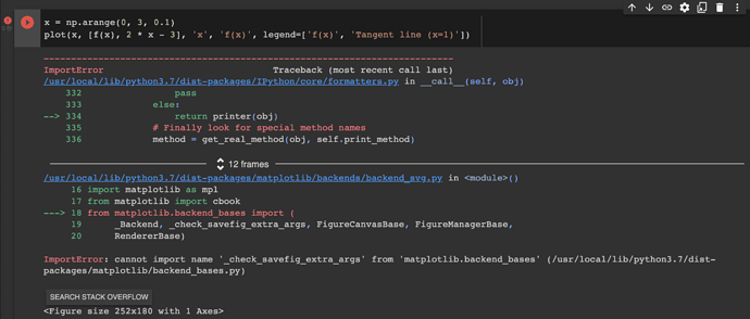
I found some issue, while I run the below code in pytorch.
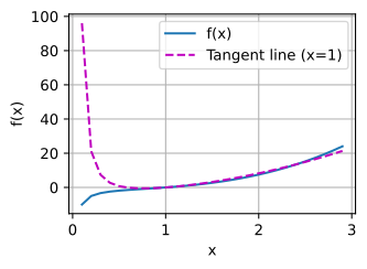
    x = np.arange(0, 3, 0.1)
    plot(x, [f(x), 2 * x - 3], 'x', 'f(x)', legend=['f(x)', 'Tangent line (x=1)'])
Thanks @zgpeace for raising this, I believe it was recently deprecated but shouldn’t error out. You can try with an older version of ipython. In any case we’ll fix this in the next release https://github.com/d2l-ai/d2l-en/pull/2065
Thank you @anirudh . I try to install d2l without version. !pip install d2l It works.
MrBean
June 29, 2022, 3:29am
28
For question one:
def f(x):
    return x ** 3 - 1.0 / x

def df(x):
    return 3 * x ** 2 + 1/ (x * x)

def tangentLine(x, x0):
    """x is the input list, x0 is the point we compute the tangent line"""
    y0 = f(x0)
    a = df(x0)
    b = y0 - a * x0
    return a * x + b

x = np.arange(0.1, 3, 0.1)
plot(x, [f(x), tangentLine(x, 2.1)], 'x', 'f(x)', legend=['f(x)', 'Tangent line (x=2.1)'])
the calculus.ipynb notebook kernel dies each time I run:
x = np.arange(0, 3, 0.1)
plot(x, [f(x), 2 * x - 3], 'x', 'f(x)', legend=['f(x)', 'Tangent line (x=1)'])
What am I supposed to do here? Thanks
Would the idea be to use a ‘generalized’ chain rule and express du/da, and du/da (something like the gradient)
du/da = f’(dx/a) + f’(dy/da) + f’(dz/da)
Maxim
December 3, 2022, 7:43am
31
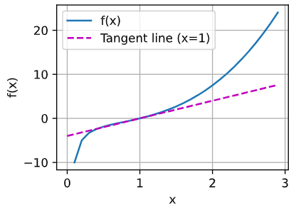
tx = 3 * x ** 2 + (1 / x ** 2) - 4
In section 2.4.3, you define gradient of a multivariate function assigning vector x to a scalar y.
At the end of the section, you give rules for gradients of matrix-vector products (which are matrices, not scalars).
I think it would help to define gradient of a matrix.
I agree with this, felt like these big topics just got skipped over
cclj
July 13, 2023, 7:44am
35
GoM
July 24, 2023, 3:47pm
38
Thanks for a great course!
Any idea regarding Q10?
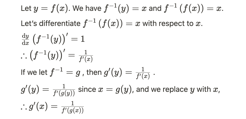
I used the given definitions as hinted - denote g=f^(-1), I was able to derive that
\frac{dg}{dx} = \frac{\frac{dg}{df}\frac{df}{dx}}{\frac{df}{dg}}
Is that the expected solution?
I think the answer of Q10 is…
1 Like
filipv
June 13, 2024, 9:07pm
41
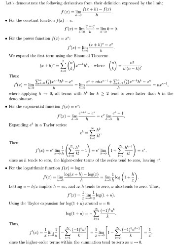
This forum won’t let me upload a pdf – if you’re interested in looking at my solutions, you’ll have to compile the LaTeX below.
\documentclass{article}
\usepackage{amsmath}
\usepackage{amssymb}

\begin{document}

\section*{Problem 1}

For $f(x) = c$ where $c$ is a constant, we have

$$
\lim_{h \to 0} \frac{f(x + h) - f(x)}{h} = \lim_{h \to 0} \frac{c - c}{h} = 0
$$

For $f(x) = x^n$, we have

\begin{equation}
\begin{split}
  \frac{df}{dx} &= \lim_{h \to 0} \frac{(x + h)^n - x^n}{h} \\
  &= \lim_{h \to 0} \frac{\binom{n}{0}x^nh^0 + \binom{n}{1}x^{n-1}h^1 + \binom{n}{2}x^{n-2}h^2 + \cdots - x^n}{h} \text{ via the binomial expansion} \\
  &= \lim_{h \to 0} \binom{n}{1}x^{n-1}h^0 + \binom{n}{2}x^{n-2}h^1 + \cdots \text{ after cancelling $x^n$ and dividing by $h$} \\
  &= \boxed{nx^{n-1}} \text{ since all terms with $h$ approach 0} \\
\end{split}
\end{equation}

For $f(x) = e^x$, we have

\begin{equation}
\begin{split}
  \frac{df}{dx} &= \lim_{h \to 0} \frac{e^{x + h} - e^x}{h} \\
  &= \lim_{h \to 0} \frac{e^xe^h - e^x}{h} \\
  &= \lim_{h \to 0} \frac{e^x(e^h - 1)}{h} \\
  &= e^x \times \lim_{h \to 0} \frac{e^h - 1}{h} \\
  &= e^x \times 1 \text{by L'Hopital's rule} \\
  &= \boxed{e^x} \\
\end{split}
\end{equation}

For $f(x) = \log(x)$

\begin{equation}
\begin{split}
  \frac{df}{dx} &= \lim_{h \to 0} \frac{\log(x + h) - \log(x)}{h} \\
  &= \lim_{h \to 0} \frac{\log\left(\frac{x + h}{x}\right)}{h} \\
  &= \lim_{u \to 0} \frac{\log\left(1 + u\right)}{ux} \text{ with } u = \frac{h}{x} \\
  &= \frac{1}{x} \lim_{u \to 0} \frac{\log(1 + u)}{u} \\
  &= \frac{1}{x} \lim_{u \to 0} \frac{1}{(1 + u)\ln{10}} \text{ by L'Hopital's rule} \\
  &= \boxed{\frac{1}{x\ln{10}}} \\
\end{split}
\end{equation}

This proof is a bit circular since it uses the derivative of $\log(x)$ when applying L'Hopital's rule! If you found a better proof, let me know.

\section*{Problem 2}

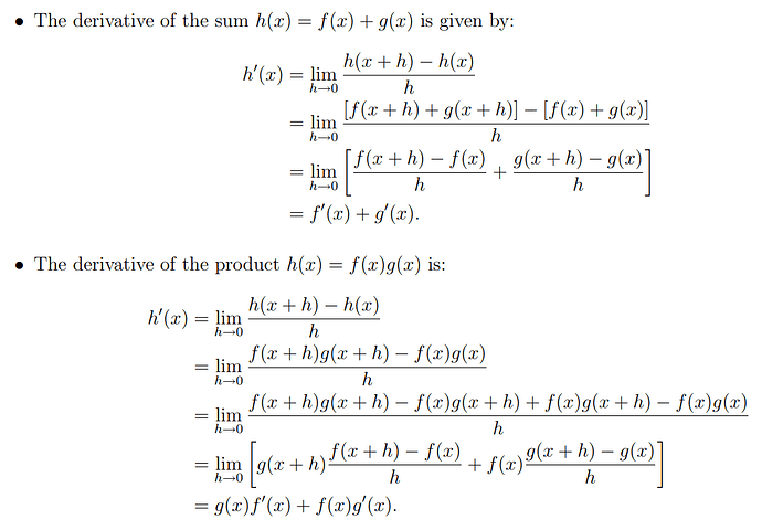
For the product rule:

\begin{equation}
\begin{split}
&\text{Prove } \frac{d}{dx} \left[ f(x)g(x) \right] = f(x)g'(x) + g(x)f'(x) \\
&= \lim_{h \to 0} \frac{f(x+h)g(x+h) - f(x)g(x)}{h} \text{ using the definition of a derivative} \\
&= \lim_{h \to 0} \frac{f(x+h)g(x+h) - f(x+h)g(x) + f(x+h)g(x) - f(x)g(x)}{h} \\
&= \lim_{h \to 0} \frac{f(x+h)\left[g(x+h)-g(x)\right] + g(x)\left[f(x+h)-f(x)\right]}{h} \\
&= f(x+0)\lim_{h \to 0} \frac{g(x+h)-g(x)}{h} + g(x)\lim_{h \to 0} \frac{f(x+h)-f(x)}{h} \\
&= \boxed{f(x)g'(x) + g(x)f'(x)} \\
\end{split}
\end{equation}

For the sum rule:

\begin{equation}
\begin{split}
&\text{Prove } \frac{d}{dx} \left[ f(x)+g(x) \right] = f'(x) + g'(x) \\
&= \lim_{h \to 0} \frac{[f(x+h)+g(x+h)] - [f(x)+g(x)]}{h} \\
&= \lim_{h \to 0} \frac{f(x+h) - f(x)}{h} + \lim_{h \to 0} \frac{g(x+h) - g(x)}{h} \\
&= \boxed{f'(x) + g'(x)} \\
\end{split}
\end{equation}

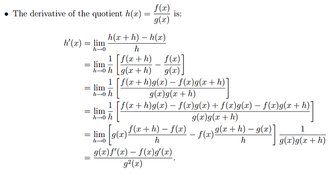
For the quotient rule:

\begin{equation}
\begin{split}
&\text{Prove } \frac{d}{dx} \left( \frac{f(x)}{g(x)} \right) = \frac{g(x)f'(x) - f(x)g'(x)}{g^2(x)} \\
&= \lim_{h \to 0} \frac{\frac{f(x+h)}{g(x+h)} - \frac{f(x)}{g(x)}}{h} \\
&= \lim_{h \to 0} \frac{f(x+h)g(x) - f(x)g(x+h)}{hg(x)g(x+h)} \\
&= \lim_{h \to 0} \frac{f(x+h)g(x)-f(x)g(x)+f(x)g(x)-f(x)g(x+h)}{hg(x+h)g(x)} \\
&= \lim_{h \to 0} \frac{g(x)[f(x+h)-f(x)] - f(x)[g(x+h)-g(x)]}{hg(x)g(x+h)} \\
&= \boxed{\frac{f'(x)g(x) - f(x)g'(x)}{g(x)^2}} \\
\end{split}
\end{equation}

\section*{Problem 3}

The product rule states $\frac{d}{dx}[f(x)g(x)] = f(x)g'(x) + g(x)f'(x)$. Let $g(x) = c$.

$$
f(x)\frac{d}{dx}c + c\frac{d}{dx}f(x) = f(x)\cdot0 + c\frac{d}{dx}f(x) = \boxed{c\frac{d}{dx}f(x)}
$$

\section*{Problem 4}

\begin{equation}
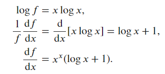
\begin{split}
y &= x^x \\
\ln{y} &= \ln{x^x} = x\ln{x} \\
\frac{1}{y}\cdot\frac{dy}{dx} &= \ln{x} + x \cdot \frac{1}{x} \text{ by the product rule} \\
\frac{dy}{dx} &= y(\ln{x} + 1) \\
\frac{dy}{dx} &= x^x(\ln{x} + 1) \\
\end{split}
\end{equation}

\section*{Problem 5}

$f(x)$ has a slope of 0 at that point. For instance, $f(x) = x^2$ has a slope of 0 at $x = 0$.

\section*{Problem 6}

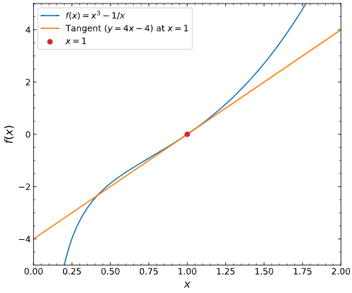
Done using $3x^2 + \frac{1}{x^2}$ to calculate the slope, yielding the final equation $4x-4$.

\section*{Problem 7}

$$
\nabla_x f(x) =
\begin{bmatrix}
  6x_1 \\
  5e^{x_2} \\
\end{bmatrix}
$$

\section*{Problem 8}

\begin{equation}
\begin{split}
  f(\mathbf{x}) &= \|\mathbf{x}\|_2 \\
  \nabla_{\mathbf{x}} \|\mathbf{x}\|_2 &= \nabla_{\mathbf{x}} (\mathbf{x}^{\top}\mathbf{x})^{1/2} \\
  &= 2\mathbf{x} \cdot \frac{1}{2}(\mathbf{x}^{\top}\mathbf{x})^{-1/2} \\
  &= \boxed{\frac{\mathbf{x}}{\|\mathbf{x}\|_2}} \\
\end{split}
\end{equation}

At $x=0$, the gradient is undefined.

\section*{Problem 9}

$$
\frac{\partial{u}}{\partial{a}} = \frac{\partial{u}}{\partial{x}} \cdot \frac{\partial{x}}{\partial{a}} + \frac{\partial{u}}{\partial{y}} \cdot \frac{\partial{y}}{\partial{a}} + \frac{\partial{u}}{\partial{z}} \cdot \frac{\partial{z}}{\partial{a}}
$$

\section*{Problem 10}

\begin{equation}
\begin{split}
y &= f^{-1}(x) \\
x &= f(y) \\
1 &= f'(y) \cdot \frac{dy}{dx} \\
\frac{dy}{dx} &= \frac{1}{f'(y)} \\
\frac{d}{dx}f^{-1}(x) &= \frac{1}{f'(f^{-1}(x))} \\
\end{split}
\end{equation}

\end{document}
Sarah
June 18, 2024, 7:10pm
42
import numpy
import matplotlib.pyplot as plt

# Code omitted to make the graph look nice: `plt.rcParams.update...`

def f(x):
    return x ** 3 - 1 / x

def df(x):
    return 3 * x ** 2 + 1 / x ** 2

def tangent(x, x_0):
    return df(x_0) * (x - x_0) + f(x_0)

x_0 = 1
x = np.arange(0.01, 2, 0.01)

_, ax = plt.subplots()
ax.plot(x, f(x), label="$f(x) = x^3 - 1/x$")
ax.plot(x, tangent(x, x_0), label="Tangent $(y = 4x - 4)$ at $x=1$")
ax.scatter(x_0, tangent(x_0, x_0), zorder=10, color="tab:red", label="$x=1$")
ax.set(xlabel="$x$", ylabel="$f(x)$", xlim=(0, 2), ylim=(-5, 5))
ax.legend();
Source: Inverse function theorem .
2 Likes
