http://d2l.ai/chapter_convolutional-neural-networks/lenet.html
“Each 2×2 pooling operation (stride 2) reduces dimensionality by a factor of 4 via spatial downsampling”. From 28x28 to 14x14, how does it reduce by a factor of 4? Since the dimensionality of a matrix is rows x cols, is it, 28x28=784; 14x14=196, hence 784-196=588 and 588 is divisible by 4, so it reduces by a factor of 4? Sorry for asking a silly question.
Hey @rezahabibi96, your question is not silly at all. Asking question is always better than keeping quiet! The origin size is 28x28=784, and the after pooling size is 14x14=196. If we calculate 784 / 196 = 4, that is where the factor “4” coming from!
2 Likes
How would we do #4 for the exercises in 6.6?
“display the activation functions” (ie sweaters and coats)?
Can we just interject visualize_activation(mx.gluon.nn.Activation('sigmoid')) somewhere and it work?
Hey @smizerex, sorry for a bit confusing here. It was asking “Display the features after the first and second convolution layers of LeNet for different inputs (e.g., sweaters and coats).” Let me know if that makes sense to you.
The input was 28x28 , We are applying a 2x2 pooling operation of stride 2 , Here stride simply means how many cells were shifted horizontally after the first pooling and vertically after the first horizontal pooling is finished . The output after performing pooling is 14x14,
The formula behind is (28-2)/2+1=14
Here 1 is the bias term and the denominator term denotes the stride .So we finally get a output of size 14x14.
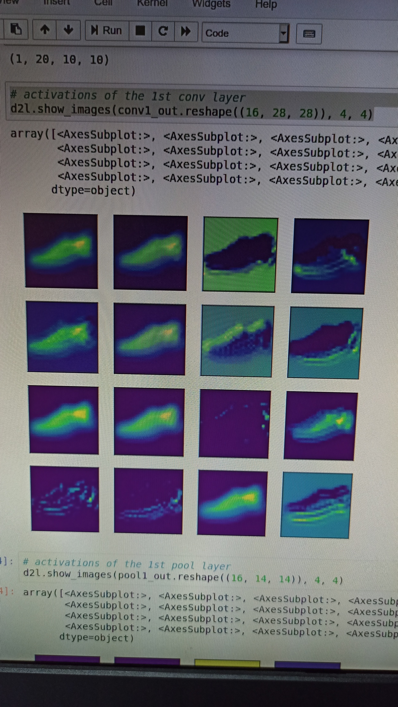
I have a problem with the activations of the first two conv layers; it appears that the first layer shows sort of a complete object (e.g. shoe) rather than showing edges. I understand that the first layers are meant to capture simple features like edges??!
Hi @osamaGkhafagy, excellent question! In general, the earlier layers try to capture the local features (such as the edge by the color contrast). However, it doesn’t need to be necessary an edge, it can be any low level coarse features for the later layers to learn.
2 Likes
Getting the following error when trying to use the gpu with mxnet:
AttributeError: 'NoneType' object has no attribute 'Pool'
system info:
(net) [six:~/code/d2l/ch6]$ cuda-memcheck --version                                                                                                                                                     (master✱)
CUDA-MEMCHECK version 10.0.130 ID:(46)
(net) [six:~/code/d2l/ch6]$ pip freeze | grep mxnet                                                                                                                                                     (master✱)
mxnet-cu100==1.7.0
(net) [six:~/code/d2l/ch6]$ nvidia-smi
+-----------------------------------------------------------------------------+
| NVIDIA-SMI 460.32.03    Driver Version: 460.32.03    CUDA Version: 11.2     |
|-------------------------------+----------------------+----------------------+
...
The relevant mxnet code is:
    def __del__(self):
        if self._worker_pool:
            # manually terminate due to a bug that pool is not automatically terminated
            # https://bugs.python.org/issue34172
            assert isinstance(self._worker_pool, multiprocessing.pool.Pool)
            self._worker_pool.terminate()
Full error output:
...
<Figure size 350x250 with 1 Axes>
<Figure size 350x250 with 1 Axes>
loss 0.471, train acc 0.823, test acc 0.829
42935.9 examples/sec on gpu(0)
Exception ignored in: <function DataLoader.__del__ at 0x7f77bcbf3d08>
Traceback (most recent call last):
  File "<local-path>/mxnet/gluon/data/dataloader.py", line 656, in __del__
AttributeError: 'NoneType' object has no attribute 'Pool'
The program completes running seemingly successfully and then dies at the assert. Seems like this is a known issue from the bug comment in the code, just wondering if there’s a workaround?
Torch seems to run lenet fine on my gpu in case that helps anyone else.
How would you go about a max-activation plot with our LeNet here?
Hello six,
I think the goal is to display is issued from each conv. layer.
Here is the call to the function I used for the display :
#-------------------------------------------------------------------------------
#Select number of sampled input-data to be processed as features-map
#-------------------------------------------------------------------------------
nb_sample=4#-------------------------------------------------------------------------------
#Select deepness of conv. net, leading to netconv, layers of convolutional process
#-------------------------------------------------------------------------------
list_layer = [0,1,2,3]
#--------------------------------------------------------------------------------
#Then call to the display function
#--------------------------------------------------------------------------------
display2D_netOutput(net, list_layer, X_test, y_test, nb_sample , is_prediction=True)
import matplotlib.image as mpimg
import matplotlib.pyplot as plt

def display2D_netOutput(net, list_layer, X_test, y_test, nb_sample , is_prediction = False, figsize=(5,5)) :
    '''Display a grid of pictures resulting in the processing of images with a trained convolutional network.
    Image is feeded into convolutional layer and result is displayed for each layer.
    Each row from grid of display matches with a layer.

    INPUT
        * net           : convolutional network containing
        * list_layer    : list of layers after which images are displayed
        * X_test        : image to be displayed.
        * y_test        : labels of images
        * nb_sample     : number of images to be displayed
        * is_prediction : when True, this flag allows to display images issued from each layer.
        * figsize       : diaplay panel shape

     OUTPUT : none
    '''

    nb_layer = len(list_layer)
    #-----------------------------------------------------------------------
    # Define grid of bounding box where pictures take place
    #-----------------------------------------------------------------------
    f, axarr = plt.subplots(nb_layer, nb_sample)
    _=plt.figure(figsize=figsize)

    #-----------------------------------------------------------------------
    # Get labels matching with X_test samples
    #-----------------------------------------------------------------------
    list_label = d2l.get_fashion_mnist_labels(y_test)

    for i_layer in range(nb_layer) :
        #-------------------------------------------------------------------------------
        # Get all layers from net until limit i_layer, start counting from 1st layer
        #-------------------------------------------------------------------------------
        netconv = net[:i_layer]

        #-------------------------------------------------------------------------------
        # Input data :
        # Get shape of input data and aggregate the samples as input data in a list.
        # Each sample from batch is reshaped as (1,nb_channels,t_shape_inputData)
        # This reshape allows to feed netconv.
        # Each feature-map is agregated into a list.
        #
        # For each input data element from batch (sized as batch_size) :
        #    * Get feature-maps using netconv; input data is reshaped to be tensor
        #      formated as (1, nb_channels, heigth, width)
        #-------------------------------------------------------------------------------
        t_shape_inputData =(X_test.shape[-2], X_test.shape[-1])
        list_X_hat = [ netconv(X_test[i_sample].reshape((1,1)+t_shape_inputData)) for i_sample in range(nb_sample)]


        #-------------------------------------------------------------------------------
        # Output data :
        # Get shape of 2D feature-map to be displayed : they are last 2 dimensions
        # of feature map.
        # The 1st feature-map from list allows to calculate feature-map shape.
        #-------------------------------------------------------------------------------
        t_shape_outputData =(list_X_hat[0].shape[-2], list_X_hat[0].shape[-1])
        X_hat_reshaped = list_X_hat[0][0][0].reshape(t_shape_outputData)


        for i_sample in range(nb_sample) :
            #-------------------------------------------------------------------------------
            # Aggregate feature-maps with bitwise sum over all of them
            #-------------------------------------------------------------------------------
            X_sum = np.zeros(t_shape_outputData)

            X_feature_map = list_X_hat[i_sample]
            nb_feature = X_feature_map[0].shape[0]

            for i_feature in range(nb_feature) :
                X_sum += X_feature_map[0][i_feature]

            axarr[i_layer,i_sample].set(label=list_label[i_sample])

            axImage = axarr[i_layer,i_sample].imshow(X_sum.asnumpy().reshape(t_shape_outputData))
            if 0 == i_layer :
                axarr[i_layer,i_sample].text(0, -2, list_label[i_sample], bbox={'facecolor': 'white', 'pad': 2})
    if is_prediction :
        y_pred = d2l.get_fashion_mnist_labels(d2l.argmax(net(X_test[:nb_sample]), axis=1))
        for i_sample in range(nb_sample) :
            axarr[nb_layer-1,i_sample].text(0, 7, list_label[i_sample], bbox={'facecolor': 'white', 'pad': 2})


    plt.show()
1 Like
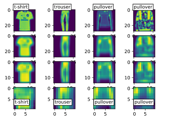
Each row matches with a layer from conv network.
First row matches with output images from first layer as last row match output images from upper conv layer block.
I think that resolution degradation as process progress through layers (this is opposite result that is expected) is due to the fact feature -maps shape decrease while display resolution stay same. This as as a zoom effect.
1 Like
@FBT Thanks for the detailed reply!
I was in fact able to answer the last question, but am asking about something slightly different – max activation plots.
In case you’re not familiar, a max activation plot, to my knowledge, is when one seeds the final layer with a spike on the category they wish to analyze and propagates the signal backwards through the net and prints out the resulting activations.
Fashion Mnist Example:
Let’s say we’d like to see what the layer plots look like when we input a “pure” t-shirt signal:
recall our categorical output vector:
['t-shirt',
 'trouser',
 'pullover',
 'dress',
 'coat',
 'sandal',
 'shirt',
 'sneaker',
 'bag',
 'ankle boot']
So we input:
[1, 0, 0, 0, 0, 0, 0, 0, 0, 0]
Hope this makes sense!
Please let me know if you or anyone else knows how to accomplish this.
Best
Six
Sidenote: Which editor/plugin do you use for those aesthetic comment lines? vim-snips perhaps?
Sorry for my confusion ! Thanks for your explanations.
1 Like
I simply use the character ‘>’ or ‘>>’ before text that leads to format it as for mardown language.
1 Like
I need datasets of both cover & stego color image to train my CNN model so it that can differentiate between them.
Horrible, horrible performance using GPU. Cuda is only working at 10% its maximum capacity.