ccpvirus

my solution to question 5

import numpy as np
from d2l import torch as d2l
x = np.linspace(- np.pi,np.pi,100)
x = torch.tensor(x, requires_grad=True)
y = torch.sin(x)
for i in range(100):
y[i].backward(retain_graph = True)

d2l.plot(x.detach(),(y.detach(),x.grad),legend = ((‘sin(x)’,“grad w.s.t x”)))

2 replies

icetea

I think it would be cool if in section 2.5.1 (and further where it occurs) there would be something like this $\frac{d}{dx}[2x^Tx]$.

rammy_vadlamudi

Any take on this question

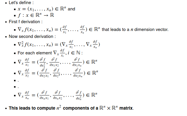
Why is the second derivative much more expensive to compute than the first derivative?

I know second derivatives could be useful to give extra information on critical points found using 1st derivative, but how does 2nd derivatives are expensive ?

2 replies

StevenJokes

@rammy_vadlamudi

chain rule

asadalam

My solution:

from mxnet import np, npx
npx.set_np()
from mxnet import autograd
def f(x):
      return np.sin(x)

x = np.linspace(- np.pi,np.pi,100)
x.attach_grad()
with autograd.record():
        y = f(x)
    
y.backward()
d2l.plot(x,(y,x.grad),legend = [('sin(x)','cos(x)')])

1 reply

StevenJokes

@asadalam
You can use or a github URLto show code…
And we should aviod import torch and mxnet at the same time…
It is confusing…

1 reply

asadalam

Any specific reason not to use both torch and mxnet and how can we use the functions like attach_grad() and build a graph without using mxnet and only simple numpy ndarrays?

1 reply

StevenJokes

@asadalam
For your first question, the reason is that in your code, you didn’t use anything related to pytorch.
So it is unnecessary to import torch
For your second question,
https://mxnet.apache.org/versions/1.6/api/python/docs/api/autograd/index.html#mxnet.autograd.backward
Check for source code

I don’t understand now…

What does these mean?
@szha

1 reply

asadalam

Oh yes, sorry, I initially used torch to use it’s sine function but couldn’t integrate with attach_grad and building the graph. Switched to numpy function but forgot to remove import torch

1 reply

StevenJokes

You can try pytorch code too. It will work.

melis

I did a few examples and discovered a problem:

from mxnet import autograd, np, npx
import math # function exp()
npx.set_np()
x = np.arange(5)
print(x)
def f(a):
    # return 2 * a * a # works fine
    return math.exp(a) # produces error
print(f(1)) # shows 2.78181...
x.attach_grad()
print(x.grad)
with autograd.record():
    fstrich = f(x)
fstrich.backward()
print(x.grad)

works fine with the function 2xx (or other polynoms) but produces error with exp(x)
TypeError: only size-1 arrays can be converted to Python scalars

[0. 1. 2. 3. 4.]
2.718281828459045
[0. 0. 0. 0. 0.]
---------------------------------------------------------------------------
TypeError                                 Traceback (most recent call last)
<ipython-input-78-cea180af7b0c> in <module>
     11 print(x.grad)
     12 with autograd.record():
---> 13     fstrich = f(x)
     14 fstrich.backward()
     15 print(x.grad)

<ipython-input-78-cea180af7b0c> in f(a)
      6 def f(a):
      7     # return 2 * a * a # works fine
----> 8     return math.exp(a) # produces error
      9 print(f(1)) # shows 2.78181...
     10 x.attach_grad()

c:\us....e\lib\site-packages\mxnet\numpy\multiarray.py in __float__(self)
    791         num_elements = self.size
    792         if num_elements != 1:
--> 793             raise TypeError('only size-1 arrays can be converted to Python scalars')
    794         return float(self.item())
    795 

TypeError: only size-1 arrays can be converted to Python scalars

I have no idea, why exp() doesn’t work.

VolodymyrGavrysh

FBT

Hello,
For the question :
“Why is the second derivative much more expensive to compute than the first derivative?”

One answer :
This is due to the fact that second derivation lead to compute N² elements from a matrix.
Please check details below.

FBT

Hello,

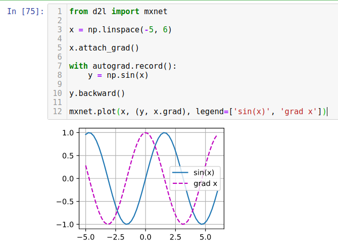
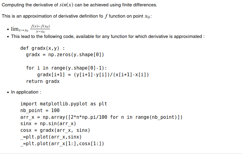
Plot sin(x) and derivative of sin(x) without the use of analytic form of the derivative can be achieved without the use of automatic differentiation framework provided by mxnet or pytorch, such as explained below :

FBT

The two plots lead to the follwings graphics :

Kem

I really dont understand Automatic Differentiation. Up until this topic, everything was intuitive and understanding for me. But i am kind of stuck here. Can i get a detailed explanation what Automatic DIfferentiation is used for. And the code is also not clear for me.

1 reply

FBT

@Kem

Automatic differentiation allows :

1. to automaticaly calculate the derivative of a function and
2. apply the resulted function to a given data.

E.g, suppose you use F(x) = 2sin(3x)* and you want to get the derivative of F for the value (array form) A=[1.,12.]

For doing so, you manually you calculate F’(x) = 6cos(3x) and then you apply value of A to the derivative, leading to [6cos(3), 6cos(36)]

Automatic differentiation avoid you to implement and calculate F’(A).

Just attaching the operator gradient to the x variable, with instruction x.attach_grad(), automatically triggers derivative operations as described just above :

1. the calculation of derivative F’(x) = 6cos(3x) and
2. the calculation of the value of A for this derivative : F’([1.,12.]) = [6cos(3), 6cos(36)]

This considerably ease the implementation of code with derivative operations, such as in back propagation.

Trishit_Mondal

Exercise 5 in Tensorflow

import math
import numpy as np
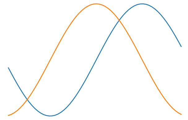
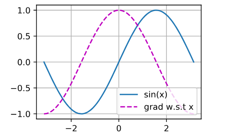
x = tf.range(-3,3,0.1)
y = np.sin(x)
d2l.plt.plot(x,y)
# gradient
with tf.GradientTape() as t:
  t.watch(x)
  p = tf.math.sin(x)
d2l.plt.plot(x,(t.gradient(p,x)))

MoradiFdev

Why python plot x*-1 around zero point as a continuous function?